Zelditch M.L. (и др.) Geometric Morphometrics for Biologists: a primer

Подождите немного. Документ загружается.

chap-10 4/6/2004 17: 26 page 238

238 GEOMETRIC MORPHOMETRICS FOR BIOLOGISTS

(A)

⫺0.025

⫺0.015

⫺0.005

0.005

0.015

0.025

0.035

3.5 4.0 4.5 5.0 5.5 6.0 6.5

PW3X

LCS

(

)

LCS

3.5 4.5 5.5 6.5

0.05

0.1

0.15

0.2

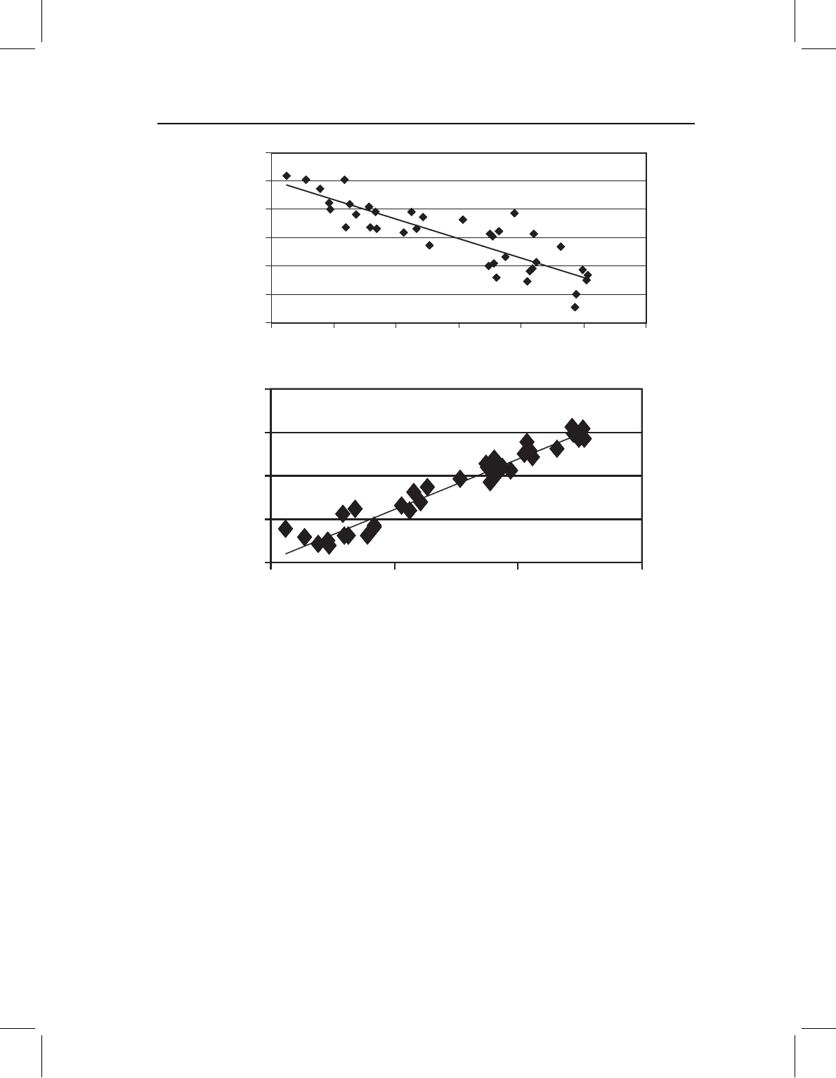
Figure 10.2 Checking the assumption of a linear relationship between shape and the independent

variable: (A) using a single variable plotted on ln centroid size; (B) using the Procrustes distance of

each specimen from the shape having the smallest size, plotted on ln centroid size.

To this point, we have talked about the assumption of linearity as it is usually stated

in bivariate regression. However, in multivariate studies there is another assumption of

linearity – the mutual linearity of all the components of the dependent variable. In other

words, we are assuming that all the components of shape are linearly related to each

other. This assumption will not hold if some components of shape are linearly related to

the independent variable, but others are non-linearly related. The components of shape

cannot be linearly related to each other if different ones fit differently shaped curves.

Because this departure from the assumption of non-linearity is specific to multivariate

data, it does not arise at all in bivariate studies, so it may not be intuitively obvious what

the assumption means. What it means is that the slope of the relationship between shape

and the independent variable is constant – the values {m

, m

,…m

} are not functions

of the independent variable.

In some cases, such as in studies of ontogeny, the shape variable correlated with age

changes from age to age. If so, we cannot model the ontogeny of shape by a single vector of

chap-10 4/6/2004 17: 26 page 239

REGRESSION 239

Uniform Y

Uniform X

⫺0.03

⫺0.04 ⫺0.02

⫺0.02

⫺0.01

0.00

0.01

0.02

0.03

0.0 0.02 0.04

One

Ten

Twenty

Thirty

Forty

Fifty

Fifteen

Twenty-five

⫺0.03

⫺0.04

⫺0.02

⫺0.01

0.01

0.02

0.03

⫺0.03 ⫺0.02 ⫺0.01 0.00 0.01 0.02 0.03 0.04 0.05 0.06

(A)

PC2

PC1

(B)

Key (ages)

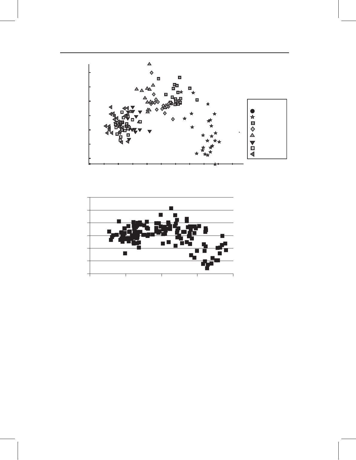
Figure 10.3 Checking the assumption of multivariate linearity of the dependent variable: (A)

using principal components analysis; (B) using two shape variables on each other (the two uniform

components).

slope coefficients because that vector changes with time. This means that the ontogenetic

trajectory of shape is a curving path in shape space, not a straight line. The assumption of

multivariate linearity can be checked in two ways, although again neither method is ideal.

One, shown in Figure 10.3, is to conduct a principal components analysis (PCA) of the

data, and check for a statistical relationship between multiple PCs and the independent

variable. In the example shown in Figure 10.3A, there is a substantial deviation from

linearity – not only is PC1 correlated with age (which we would expect), but PC2 and PC3

are also. PC2 and PC3 describe the deviations from the linear trend represented by PC1.

The assumption can also be checked by regressing several shape variables on each other

(Figure 10.3B). If the relationship among these variables is non-linear, we must reject the

assumption of multivariate linearity.

chap-10 4/6/2004 17: 26 page 240

240 GEOMETRIC MORPHOMETRICS FOR BIOLOGISTS

When shape data violate the assumption of multivariate linearity, there is no easy way

to transform them. They are not individual variables that can be individually transformed;

they all, taken together, represent a single variable – shape. If we log transform some of

the components, we thereby alter the meaning of “shape.” Also, whenever the dependent

variable is transformed, the error structure of the data is also affected (which does not hap-

pen when only the independent variable is transformed, because that variable is presumed

to be measured without error). Moreover, and perhaps most important, the non-linear

dynamics of the shape variable are not just a nuisance, they are biologically interesting

(but they do complicate statistical analyses).

Testing the null hypothesis of isometry for S. gouldingi

We checked the assumption that shape is linearly related to size over the ontogeny of

S. gouldingi in Figures 10.1 and 10.2, determining that shape is nearly linearly related to

log centroid size. We can now test the null hypothesis that the relationship between shape

and size is no greater than we would expect by chance. Our null hypothesis is isometric

growth, meaning that shape does not change as a function of size. If we can reject that null

hypothesis, we can say that shape is a function of size. Regressing the full set of partial

warps on the natural log of centroid size yields a value of Wilk’s  of 0.0109, corresponding

to an F-statistic of 29.1 with 28 and 9 degrees of freedom (p =6.07 ×10

−6

). Thus, it is

highly improbable that the null hypothesis is true. We can therefore reject it in favor of

the alternative hypothesis – that shape is allometric (meaning it changes as a function of

size). To determine the proportion of the shape variation predicted by size, we will sum the

squared Procrustes distances between the observed shape and the shape predicted for that

individual given its size. From that sum, we conclude that 28.1% of the shape variance is

not explained by the regression. Thus, 100% −28.1% =71.9% of the shape variance is

explained by size.

Using regression to compare group means

To this point we have used regression to examine the relationship between continuous

variables, but regression can also be used for comparing populations that differ categori-

cally if the categories are viewed as discrete points along an inherently continuous scale.

This application of regression requires transforming what was measured as a categorical

variable into a variable on a continuous scale, a procedure that can be tricky (and even

unjustified). We first show how it is done, then discuss when it might be justified (or not).

We will begin with a simple case, in which we are actually doing a simple two-group

analysis of variance. We assign numerical values (called “dummy codes”) to our two

groups. Typically, one is assigned a value of 1 and the other a value of −1 or 0. Then,

shape is regressed on these coded values. If the dummy codes are 1 and 0, the regression

describes the difference between groups, and the intercept is equivalent to the mean of the

group coded “0” (because the intercept, by definition, is the value for Y when X equals

zero). Alternatively, if the groups are coded by −1 and 1, the Y-intercept is located at the

mean over both groups, and the regression will show half the difference between them. The

statistical significance of the regression indicates whether there is a significant difference

between the two groups, and the test is equivalent to a generalized Hotelling’s T

test.

chap-10 4/6/2004 17: 26 page 241

REGRESSION 241

This simple case of using regression to compare two groups raises no problems, either

conceptual or statistical. It does not matter that we have transformed categorical variables

A and B into the ordinal variables −1 and 0, or 0 and 1, and used a method that presumes

these are continuous variables. However, real problems can arise when we are analyzing

more than two groups because then the codes (e.g. −1, 0, and 1) are treated as if the distance

between the integers is meaningful on a continuous scale. When we use regression, we are

calibrating the effect of a change of a given amount in X on Y; if that amount of change

in X is arbitrary, the calibration does not make sense. Thus, whether this approach is

justified or not depends on whether it makes sense to translate the categorical variable into

a continuous one.

In some cases that translation might seem reasonable, even more appropriate than

leaving the variable categorical, because the categories are arbitrary subdivisions of an

underlying continuum. For example, perhaps we subdivided a continuum of ages into

classes such as juveniles, subadults and adults. Age is a continuously valued variable and the

age classes are ordered from youngest to oldest, and we would like to take that ordering into

account when analyzing the data. Using analysis of variance we cannot take the ordering

into account, so regression might seem a superior approach to the data. However, our

ordered classes might not be separated by equal increments of time (either chronological

or developmental) – the distance from juvenile to subadult on a temporal scale might not

correspond to the distance from subadult to adult on that same scale. If that is the case

our X-axis is not meaningful, so it does not make sense to calibrate the change in shape

by the change along a meaningless scale. That objection might be subdued by finding a

strong linear relationship between shape and age class. However, it is far more difficult

to justify using this approach when we cannot view the coded variables as representing a

progression from least to most along an underlying factor.

The most problematic cases are those in which the categorical variable is complex but

we single out one component as the independent variable. For example, suppose we wish to

know whether diet has an effect on shape. To that end, we subdivide diets into “herbivore,”

“carnivore” or “omnivore,” perhaps ordering them by percentage of meat in the diet. This

approach might seem reasonable at first, but we could also order diets by hardness of food

(or even by the energy required to find it, capture it, or process it, or the net energy required

by all those activities). Hardness might be a reasonable choice, because carnivores that

crush bone might be more similar to herbivores that crush nuts than either is to carnivores

that shear flesh or to frugivores. The energy required to capture and process prey is also

a reasonable choice, because shape may matter when the costs of energetically expensive

activities can be reduced by optimizing shape. Considering that all three characterizations

of the independent variable can yield different results, we cannot equate one of them

to “diet.”

Another, more technical, issue that also makes this approach problematic is that we are

modeling the relationship between shape and the categorical variable by a straight line.

That assumes that the relationship between them is linear, and the form of the relationship

might depend largely on how we have subdivided the categories. It also assumes that

there is a meaningful distance between the classes that we have quantified with some

arbitrariness. For the distance to be meaningful, the change from 0.0 to −1.0 should be

of the same magnitude, and in the opposite direction, as the change from 0.0 to 1.0.

Moreover, the change from 1.0 to 3.0 should be in the same direction, and equal to twice

chap-10 4/6/2004 17: 26 page 242

242 GEOMETRIC MORPHOMETRICS FOR BIOLOGISTS

the magnitude, as the change from 0.0 to 1.0. To calibrate the effect of the coded states on

shape, which is what we are doing when we estimate a slope, we must have good reason to

assume that there is a linear and regular relationship between coded states. For example,

if we subdivide diets into herbivory, omnivory, and carnivory, coding them as 1, 2, and

3, we are assuming that the difference between herbivory and ominivory is equal to the

difference between omnivory and carnivory, which implies that frugivory and granivory

are equivalent (as types of herbivory). Additionally, it implies either that insectivory and

molluscivory do not occur, or that they can be classified with carnivory (on physiological

grounds). The problems we face are due to the complexity of “diet.” Like shape, it is

a multidimensional variable, so we face both the problem of transforming a complex

multidimensional variable into a simple scalar, and also the challenging task of creating

meaningful distances along the continuum. It may be more appropriate to treat complex

multidimensional factors as exactly that and use a different method (such as partial least

squares, Chapter 12) rather than regression.

The reason for raising these issues is that regression may seem like an attractive approach

to analyze ordered variables. Unlike MANOVA, it does not merely ask if discrete classes

differ. When the classes are ordered, regression may be a more appealing method. However,

it is not always an appropriate one, even when the underlying factor is continuous. To

decide whether regression is appropriate, consider whether it makes sense to treat the

dependent variable as one-dimensional, and if there is a meaningful metric along that

dimension.

Standardization

To this point, we have used regression to study the phenomenon of interest – the depen-

dence of shape on another variable (size in our example). Often that relationship is not of

primary interest, but is a nuisance that may be obscuring something more interesting. For

example, we might want to ask if two species differ in shape, when we already know that

they differ in size. We also know that size affects shape, so before comparing the species,

we want to remove the effect of size on shape. Specifically, we want to ask if they differ in

shape when the effect of size is controlled. To take a concrete example, suppose we wish

to compare the shapes of S. gouldingi and S. manueli; and, as we have already shown, the

shape of S. gouldingi depends highly on size (the same is true for S. manueli). If we were

fortunate enough to have large samples of comparably sized specimens of both species (so

that the mean size is the same for both), we could compare their mean shapes directly.

However, the average body size in our sample of S. gouldingi is 177.99 mm whereas it is

108.95 mm in our sample of S. manueli, so it is possible that any differences we might find

between their shapes is due to the impact of size on shape.

One common approach to solving this problem is to include a covariate in the analysis

of variance (thus doing an analysis of covariance, ANCOVA, or MANCOVA in the mul-

tivariate case). The null hypothesis of an ANCOVA is that the groups (the two species in

our case) do not differ after we take the covariate into account. In effect, we will remove

the shape variance predicted by the covariate (size, in our example) and ask if the mean

shapes differ. That is done by fitting both species to the same regression line (meaning

the slopes are the same for both species) and comparing their values of {b

, b

,…b

}

chap-10 4/6/2004 17: 26 page 243

REGRESSION 243

Size Size

(A) (B)

Shape

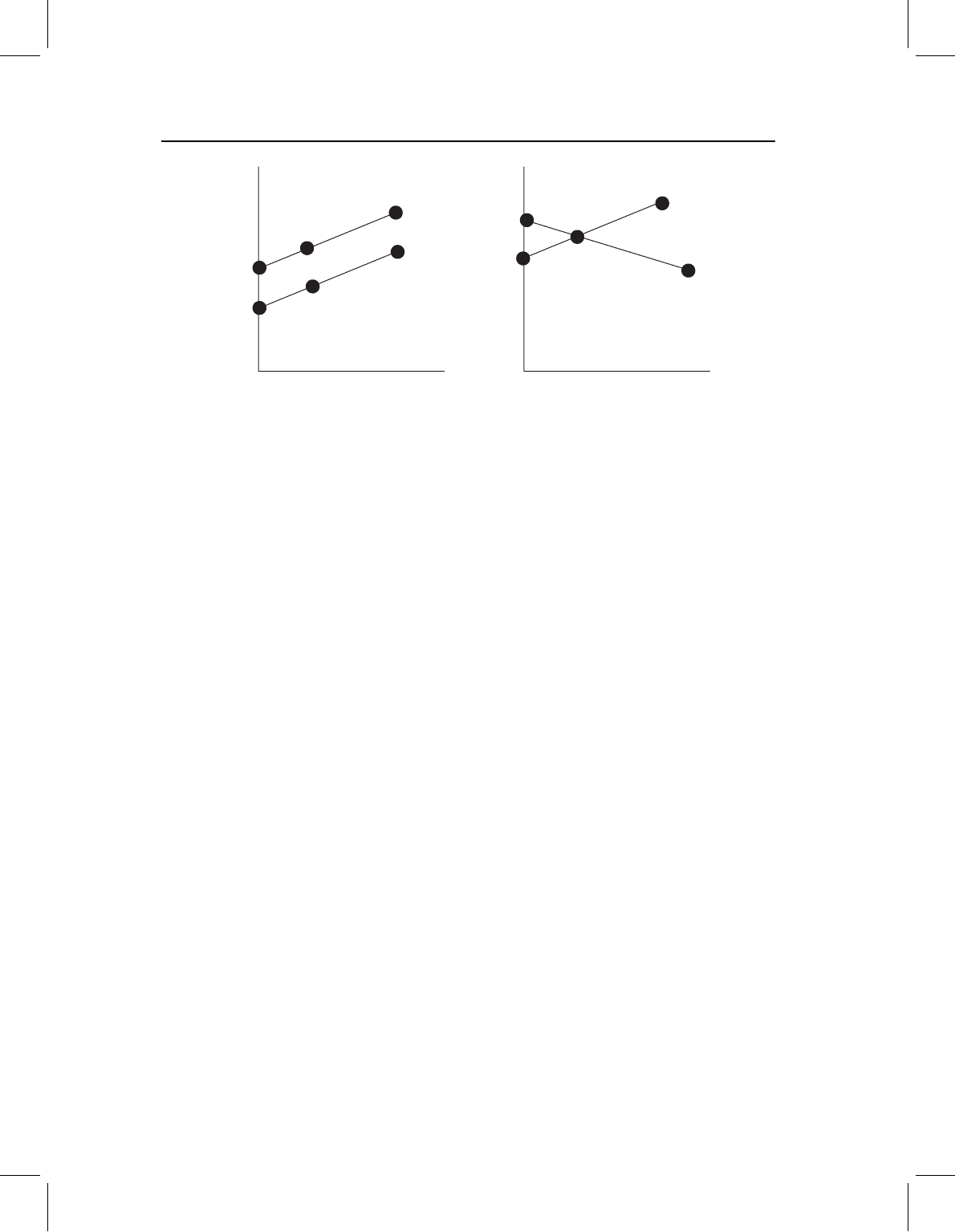
Figure 10.4 Why the assumption of common slopes matters. (A) When the slopes are the same,

the same results are obtained regardless of the value of the independent variable at which samples

are compared. (B) When the slopes differ, the results are a function of the values of the independent

variable at which samples are compared. The points on the lines indicate the shapes being compared.

Note that in (A) the same distance separates the points on the two lines over all sizes, whereas in (B)

the distance between points increases then decreases as size increases.

which gives the expected shape when the independent variable is zero. Actually, it does

not matter what size we use for the comparison – if the assumption of a common slope

holds, we will always find the same difference between the two species. The rationale for

this is shown in Figure 10.4: when the slopes are the same, the difference between the

two regression lines is constant (Figure 10.4A). It is not a function of the size at which we

compare them. In contrast, when the slopes are different, the difference between the two

groups is a function of the independent variable; the difference between the shapes of these

two groups depends on the size at which they are compared (Figure 10.4B). Because the

two lines intersect, there is a value at which their shapes are the same; but because they

intersect at just one point, there is only one point at which their shapes are the same.

The first step in any analysis of covariance (ANCOVA or MANCOVA) is to test the

null hypothesis that the slopes are the same. This null is rejected when there is a significant

interaction between the covariate (size in this case) and the factor of interest (species in

this case). In the comparison between S. gouldingi and S. manueli, the null hypothesis of a

common slope is unequivocally rejected; Wilks’  =0.151, corresponding to an F-statistic

of 9.46 with 28 and 47 degrees of freedom (p1 ×10

−6

). Clearly, it is highly improbable

that the null model is true.

At this point it might not seem necessary to pursue the analysis any further, because we

have already shown that the regression lines intersect so the difference in shape between

these two groups cannot be a simple consequence of their difference in size. Even if their

shapes are not different at some value of size, they will be at another. Nevertheless, we

might still wish to pursue the analysis further because we might want to know if they

differ at a particular size. For example, we might want to know if they are different early

in development, or just later. Just because we know that the difference in shape between

the two species depends on the size at which we compare them does not mean that we

no longer are interested in their differences at particular sizes. In ruling out the simple

chap-10 4/6/2004 17: 26 page 244

244 GEOMETRIC MORPHOMETRICS FOR BIOLOGISTS

hypothesis that the interspecific difference in shape is purely a function of the interspecific

difference in size, we have not exhausted our questions.

When slopes differ, we can still use regression to remove the effects of size but we must

remove those effects separately, group by group. Now, we have to choose the value(s)

of size at which we will compare them, because the results will depend on that choice.

We also need to decide whether to compare them at the same size or at a biologically

comparable size. If we want to interpret the shape differences in functional terms, it makes

sense to compare them at the same size; all the theories we are considering relate shape to

size. However, if we want to interpret shape differences in developmental terms, we might

prefer to compare groups at developmentally comparable stages. Different groups may

reach the same developmental stage at different sizes (and/or ages), so comparing them at

a comparable stage may require comparing them at different sizes.

Whatever size(s) we pick, the procedure is the same. We fit the data to the linear

model, predict the expected shape at a particular size, and use that expected shape in

our comparisons. The expectation is for the mean, and if we want to know whether the

difference between species is statistically significant, we need more than the estimate of

the mean. We also need to know the variation around the mean for each species. We can

estimate that from the variation around the regression line – each individual deviates from

the shape expected for its size. The residuals from the regression line are the deviations

of an individual from the mean shape expected for its size, so we can use those residuals

to estimate the variation around the expected shape at one particular size. We add those

residuals to the expected shape at a given size, creating a “model population.” The model

population has the mean shape predicted by the regression equation, and the variance

obtained from the residuals from the regression. In producing this model population we

are assuming linearity of the relationship between size and shape, and even small departures

from linearity can become important because the residuals will not be randomly distributed

around the regression line (hence they are not randomly distributed around the mean).

Also, in using the regression equation to remove the effect of one factor on shape, we are

assuming that this factor does not interact with any others.

We need to take a cautious approach to size standardization (and to standardization by

any other variable), but it is often useful when we want to know whether samples differ

in another variable, taking into account their differences in size. To exemplify both the

rationale for size standardization, as well as its impact on comparative studies, we will

compare the shapes of S. elongatus, S. gouldingi and S. manueli, first without controlling

for the effects of size, and then after standardizing them to two different sizes.

Comparing shapes of S. elongatus, S. gouldingi and S. manueli

We first ask whether these three species differ significantly in shape, and if so how and by

how much. We will use MANOVA to test the hypothesis that they do not differ in shape

(see Chapter 9), then use canonical variates analysis (CVA) to find the dimensions along

which they are optimally discriminated (see Chapter 7), and then measure the Procrustes

distance between their shapes to determine by how much they differ. Based on MANOVA,

the three species are unquestionably different in shape, Wilks’  =0.0095 corresponding

to a χ

of 500, with 56 degrees of freedom (p 1 ×10

−6

). The discriminant function

misclassifies only three of the 124 specimens (one individual of S. gouldingi is misclassified

chap-10 4/6/2004 17: 26 page 245

REGRESSION 245

⫺0.020

⫺0.015

⫺0.010⫺0.005

0.005 0.010 0.015 0.020

⫺0.010

⫺0.005

0.005

0.010

0.015

CV1

CV2

S. elongatus

S. gouldingi

S. manueli

⫺0.015

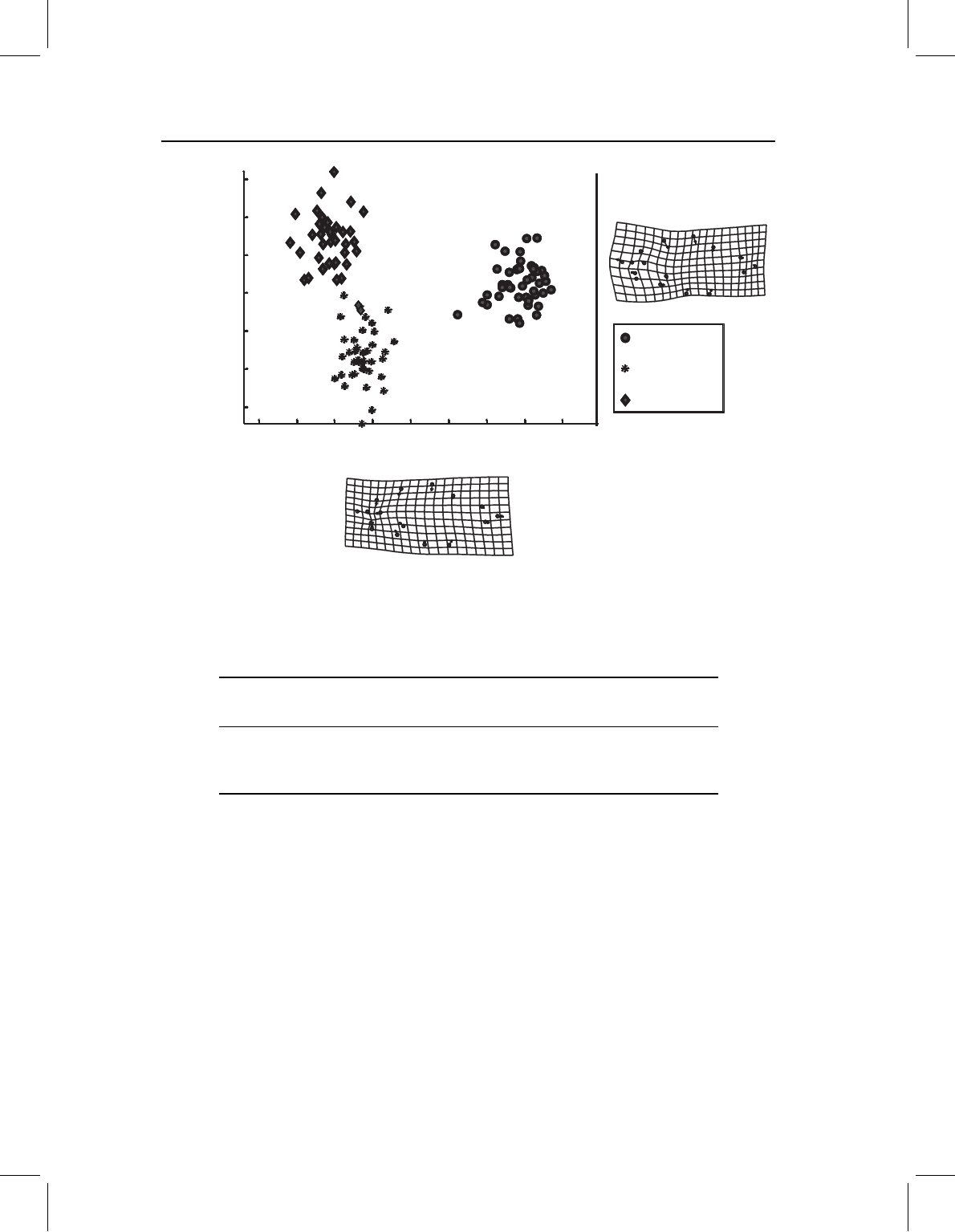
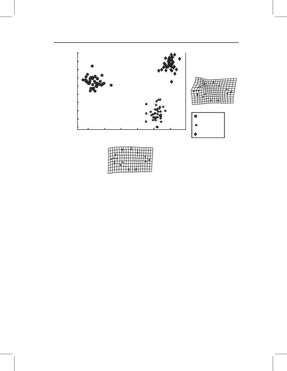
Figure 10.5 Canonical variates analysis of three species of piranhas; data are from an ontogenetic

series and are not standardized to remove the variation related to size.

Table 10.1 Procrustes distances between species, the unstandardized values are

calculated without removing the variation due to size from the data

Species Unstandardized Standardized Standardized

juveniles adults

S. elongatus vs S. gouldingi 0.079 0.060 0.126

S. gouldingi vs S. manueli 0.046 0.080 0.051

S. elongatus vs S. manueli 0.076 0.071 0.128

The distances between juvenile shapes and adult shapes are calculated after removing the

variation due to size from the data. Juvenile shapes are standardized to the size at which each

species undergoes the transition from larval to juvenile growth; adult shapes are standardized

to the maximum adult body size for each species.

as S. manueli, and two S. manueli as S. gouldingi). A posteriori tests of the pairwise

differences find that all are distinct from all others at (p < 0.001). The two dimensions

maximally distinguishing among species are shown in Figure 10.5, and the Procrustes

distances are given in Table 10.1.

We will now compare them at 20 mm standard length (SL), the size at which all three

species undergo the transition from larval to juvenile growth. We do not have specimens

of that size for either S. gouldingi or S. manueli because we have been unable, to date,

to distinguish between them at those sizes. However, analyses of other species show that

the regression of shape on size is nearly linear and that it does not tend to depart from

linearity at small values, so we will extrapolate the regression to 20 mm even though that

chap-10 4/6/2004 17: 26 page 246

246 GEOMETRIC MORPHOMETRICS FOR BIOLOGISTS

⫺0.03 ⫺0.02 ⫺0.01 0 0.01 0.02

⫺0.025

⫺0.020

⫺0.015

⫺0.010

⫺0.005

0.005

0.010

0.015

0.020

CV1

CV2

S. elongatus

S. gouldingi

S. manueli

Figure 10.6 Canonical variates analysis of three species of piranhas; data are from ontogenetic

series and are standardized to remove the variation related to size. Comparisons are made at the

transition from larval to juvenile phases.

is beyond the range of the data for these two species. Having adjusted the data for size,

we will repeat the same three analyses. Once again, we find that the three species are

unquestionably different in shape, Wilks’  =0.0013 corresponding to a χ

of 718 with

56 degrees of freedom (p 1 ×10

−6

). This time, no specimens are misclassified. The a

posteriori pairwise tests again show that all three species differ significantly from all others

in mean shapes (p < 0.001). To this point, standardization might seem to have had little

effect, other than to inform us that the differences we found above are not an artifact

of the distribution of body sizes in our samples. However, the Procrustes distances are

clearly affected by the removal of the size-related variation (Table 10.1). Based on the

unstandardized data we would conclude that S. elongatus is strikingly different from the

other two species, but based on the standardized data it appears that S. manueli and

S. gouldingi are actually more different from each other than either is from S. elongatus.

Also, the directions along which the species are optimally discriminated change when the

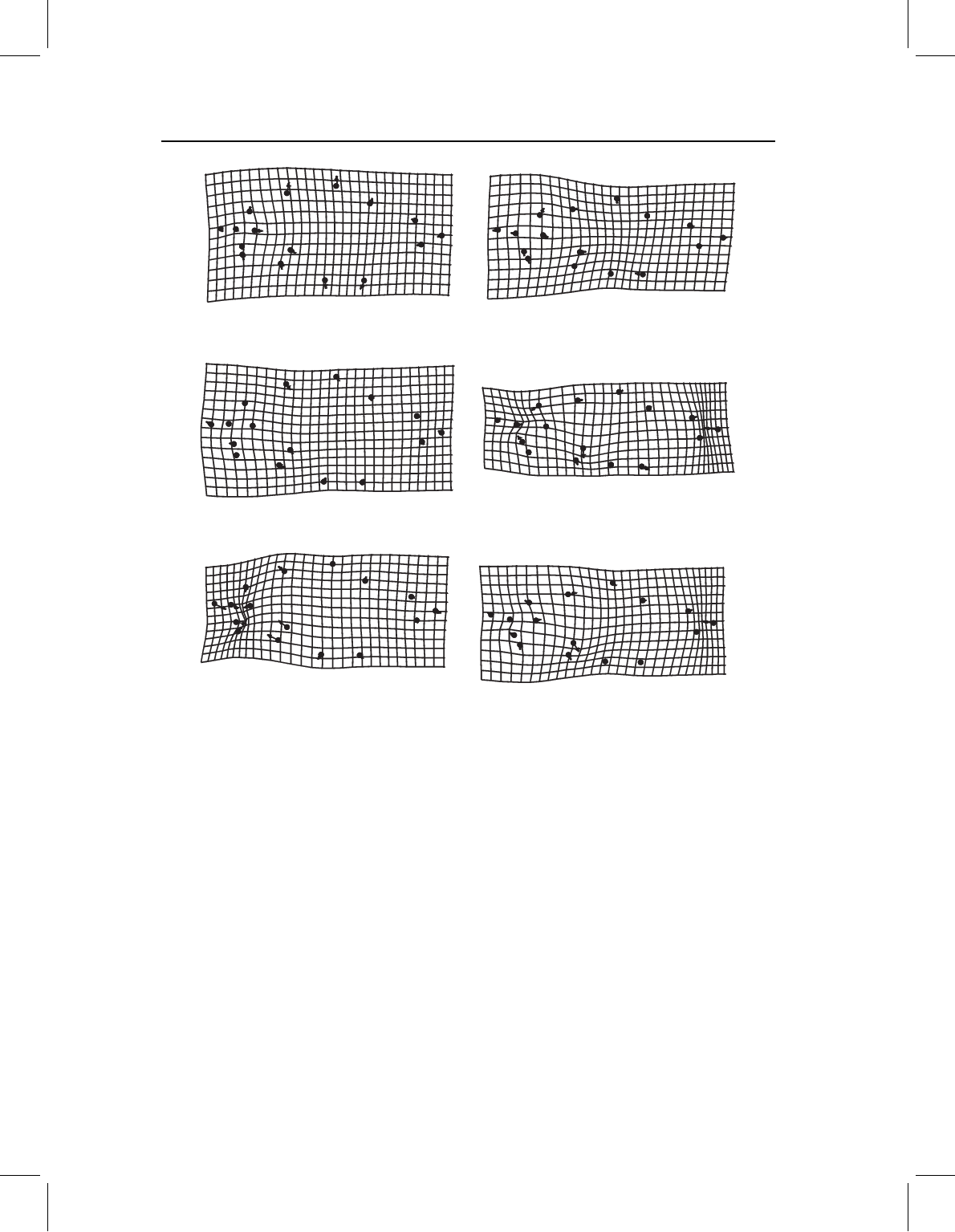
data are standardized (Figure. 10.6), and so do the directions in which pairs of species

differ (Figure 10.7).

The comparison between these three species conducted at their maximum body sizes

reveals a very different pattern. CVA at this size still reveals unequivocally significant dif-

ferentiation, with Wilk’s  =0.0014 corresponding to a χ

of 703 with 56 degrees of

freedom (p 1 ×10

−6

) and no specimens misclassified. However, the optimal discrimi-

nator is very different from that determined for both the unstandardized data and the data

chap-10 4/6/2004 17: 26 page 247

REGRESSION 247

(A)

(B)

(C)

Figure 10.7 Pairwise differences between means of unstandardized data (on the left) and the data

standardized to 20 mm SL (on the right): (A) S. elongatus vs S. gouldingi; (B) S. gouldingi vs

S. manueli; (C) S. elongatus vs S. manueli.

standardized to a small juvenile’s size (Figure 10.8), and the pairwise differences do not

resemble those found in either the standardized data (Figure 10.9) or in the comparisons

at small juvenile sizes (Figure 10.10). Also, the interspecific distances are affected both by

standardization and by the size/age at which they are compared (Table 10.1). The distance

from S. elongatus to both S. gouldingi and S. manueli is far greater when compared at the

small juvenile size than when compared at maximum adult size, and the distance between

S. gouldingi and S. manueli is far less. Although that second distance is not much greater

than that found in the unstandardized data, the ratio of the distance between S. gouldingi

and S. manueli relative to the distance between S. elongatus and each of those two species

differs dramatically.

This simple example makes two important points: one is that standardization can have

a large impact on both the magnitude and direction of a difference between groups, and

the second is that the inter-group differences are sensitive to the value of the independent

variable. This sensitivity is due to violating the assumption of a common slope. When

regression lines are parallel, it does not matter what value of X is chosen – the same