Zelditch M.L. (и др.) Geometric Morphometrics for Biologists: a primer

Подождите немного. Документ загружается.

chap-04 4/6/2004 17: 22 page 98

98 GEOMETRIC MORPHOMETRICS FOR BIOLOGISTS

We can take this example a step further by specifying that all the chairs are located along

walls of the room, with every chair touching the wall. Now, the X- and Y-coordinates

can be replaced by the distance (L) around the perimeter of the room from the door to the

notebook, and the direction of the measurement (clockwise or counter-clockwise). If we

agree that distances around a perimeter are always measured in the same direction, then the

value of L is sufficient to describe the location of the notebook. The additional constraints

(chairs against the wall, perimeter measured in clockwise direction) have reduced the

degrees of freedom from two (X and Y) to one (L). We have not actually eliminated

either X or Y; rather, we have merely replaced that pair by L. Nor have we lost any

information; given L, and the direction in which L is measured, as well as the height of

the chairs, we can reconstruct the original three Cartesian coordinates (X, Y, and Z)of

the notebook.

In the case of two-dimensional shapes, we start out with K landmarks in two dimensions,

so we have 2K coordinates, which constitute 2K independent measurements (because each

coordinate is independent of the others, in principle). In the course of superimposing the

shapes on the reference form, we perform three operations: (1) we center the matrix on the

centroid, thereby losing two degrees of freedom; (2) we set centroid size to one, thereby

losing another; and (3) we compute the angle through which to rotate the specimen, thereby

losing one more. By the end, we have lost four degrees of freedom as a consequence of

applying these constraints to the data. However, unlike the notebook example, we still

have 2K variable coordinates in our data matrix; none of them have been removed or

constrained. We have not lost degrees of freedom by removing coordinates, because the

loss of degrees of freedom is shared by all coordinates – each coordinate has lost some

fraction of a degree of freedom because each is partially constrained by the operations of

centering, scaling and rotation. Consequently, we have too many variable coordinates for

the degrees of freedom. The primary advantage of the thin-plate spline methods (discussed

in Chapter 6) is that we can work with 2K −4 variables, so that the number of variables

and the number of degrees of freedom are the same.

Summary

Because there are several different morphometric spaces and distances, some with only

slightly different names, we summarize them below.

The configuration space is the set of all matrices representing landmark configurations

that have the same number of landmarks and coordinates. This space has K ×M

dimensions, where K is the number of landmarks and M is the number of coordinates.

The pre-shape space is the set of all K ×M configurations with a centroid size of one,

centered at the origin. This space is the surface of a hypersphere of radius one. Because of

the centering, configurations that differ only in position are represented as the same point in

pre-shape space. Similarly, because of the scaling, configurations that differ only in centroid

size are represented by the same point in pre-shape space. Consequently, this space has

KM –(M +1) dimensions; M dimensions are lost due to centering, and one dimension is

lost due to scaling. In pre-shape space, the set of all configurations that may be converted

into one another by rotation lies along a circular arc called a fiber, which lies on the surface

of the pre-shape hypersphere. The distance between shapes in pre-shape space is the length

of the shortest arc across the surface connecting the fibers representing those shapes, and

chap-04 4/6/2004 17: 22 page 99

THEORY OF SHAPE 99

is called the Procrustes distance. Because the radius of the pre-shape hypersphere is one,

the length of the arc is also the value (in radians) of the angle subtended (ρ).

To construct a shape space, we select one point on each fiber, removing differences in

rotation. The number of axes on which a configuration can be rotated is a function of the

number of landmark coordinates: M(M −1)/2. This also specifies the number of dimen-

sions that are lost in the transition from pre-shape space to shape space (1 if M =2, 3 if

M =3). The construction of a shape space begins with the selection of one shape in a conve-

nient orientation to serve as the reference configuration. Every other shape (called a target

configuration) is placed in the orientation that corresponds to the location on its fiber that

is closest to the reference. This orientation is the position that minimizes the square root of

the sum of the squared differences between the coordinates of corresponding landmarks.

When minimized simply by rotation, this quantity is called the partial Procrustes distance.

Configurations that satisfy this condition are said to be in partial Procrustes superimposi-

tion on the reference. The partial Procrustes distance is the length of the chord of the arc

between the fibers in pre-shape space.

After rotation to partial Procrustes superimposition, the square root of the sum of the

squared differences between the coordinates of corresponding landmarks can be further

reduced by rescaling the target to centroid size of cos(ρ). Configurations that satisfy this

condition are said to be in full Procrustes superimposition on the reference; and the result-

ing distance between shapes (square root of the sum of the squared differences between the

coordinates of corresponding landmarks) is the full Procrustes distance. The set of shapes

in full Procrustes superimposition comprises a hypersphere of radius one-half, inside the

hypersphere of shapes in partial Procrustes superimposition, and tangent to the larger

hypersphere at the reference. This smaller, inner hypersphere is Kendall’s shape space.

Problems and exercises on the theory of shape

To get a feel for what the software will be doing for you, do these problems and exercises

using pencil, paper and a scientific calculator. The numbers of landmarks are small, to

keep the level of tedium to a minimum!

1. Suppose that the configuration matrix for a given shape is:

A =





0.0 −1.0

0.00.5

0.7 −0.2





a. How many landmarks are there in this configuration? How many dimensions does

it have?

b. Sketch the shape representing this configuration (you may want to use graph paper,

if it helps). Number the landmarks.

c. Write out the row vector form of this landmark configuration.

d. Find the centroid position of this landmark configuration. How many coordinates

are in the centroid position? Sketch the location of the centroid on your picture

from (b) above.

chap-04 4/6/2004 17: 22 page 100

100 GEOMETRIC MORPHOMETRICS FOR BIOLOGISTS

e. Write out the centered form of this configuration matrix, by subtracting the value

of the X-coordinate of the centroid from each of the values in the first column,

and subtracting the value of the Y-coordinate of the centroid from each of the

values in the second column.

f. Find the centroid size of this landmark configuration.

g. Now form the pre-shape configuration for A. Do this by dividing the centered form

of this matrix (solution to (e) above) by the centroid size (solution to (f) above).

Remember that when you divide a matrix by a scalar (an ordinary number, like

centroid size), you must divide each value in the matrix by the scalar divisor (which

is centroid size in this case).

2. Suppose a configuration of dimensional landmarks is given by:

B ={0.3, −1.0, 0.25, −0.4, 0.0, 0.75, −0.2, 0.35}

a. How many landmarks are in this configuration?

b. Write out the configuration matrix for this configuration.

c. Find the centroid for this configuration.

d. Find the centroid size for this configuration.

3. Given the landmark configuration:

C ={0.1, 0.1, 0.1, 0.3, −1.0, 1.1, −0.6, −0.3, 0.2, 0.3, −0.1, 0.15}

can you determine what K and M are?

4. Suppose we have the configuration matrix:

X =





0.50.5

−0.20.3

0.10.3





a. Compute a configuration matrix that would represent X in pre-shape space.

b. Now, for the truly stout of heart, suppose we have a second configuration matrix

in pre-shape space:

Y =





0.6864 0.1961

−0.6864 −0.0981

0.0 −0.0981





Determine the angle that you would have to rotate the pre-shape space matrix

form of X (from (a) above) to produce a partial Procrustes superposition of X on

the reference form Y.

5. Given two matrices:

X =





0.7146 0.2150

−0.6438 −0.0913

−0.0709 −0.1237





Y =





0.6864 0.1961

−0.6864 −0.0981

0.0 −0.0981





chap-04 4/6/2004 17: 22 page 101

THEORY OF SHAPE 101

where X is in partial Procrustes superposition with Y:

a. Find the partial Procrustes distance between the two.

b. Use the partial Procrustes distance to find the Procrustes distance between the two.

c. Use the Procrustes distance to calculate the full Procrustes distance between

the two.

Answers to problems and exercises

(A full solution is given if the calculation has not been seen before.)

1. Looking at the configuration matrix:

a. There are three landmarks (K =3 rows) and each is in two dimensions (M =2

columns).

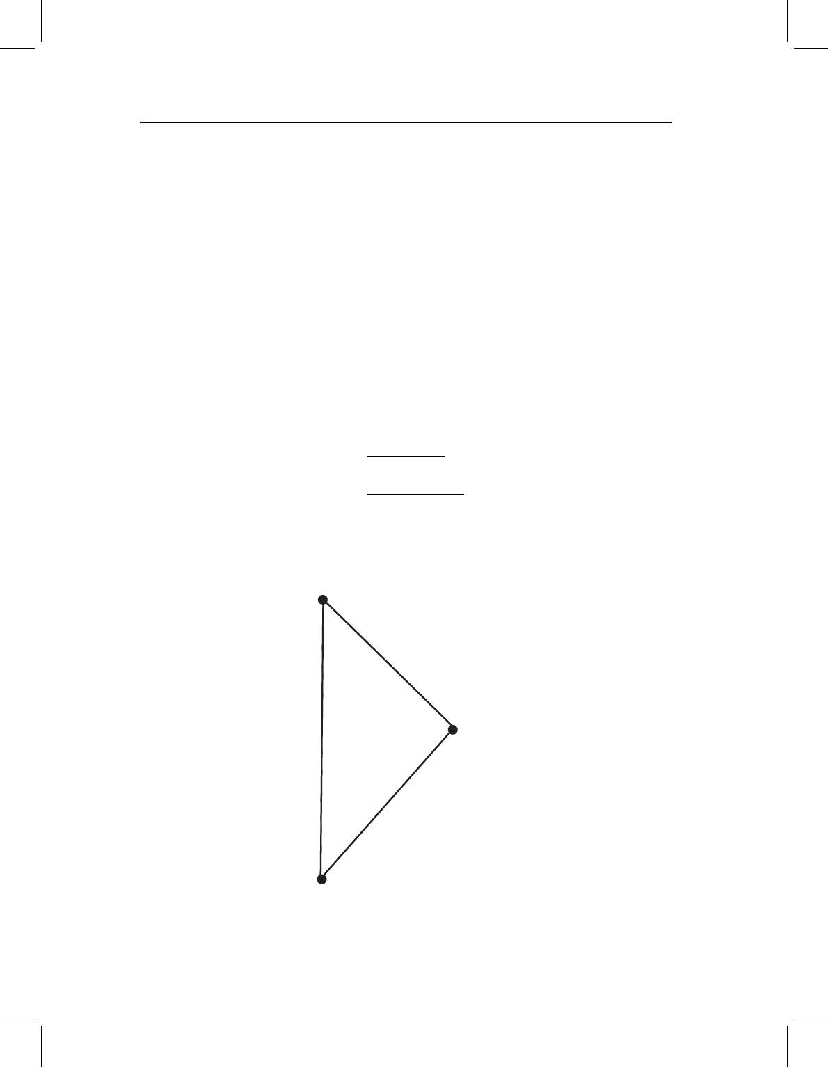
b. See Figure 4.19.

c. In row form, A ={0.0, −1.0, 0.0, 0.5, 0.7, −0.2}.

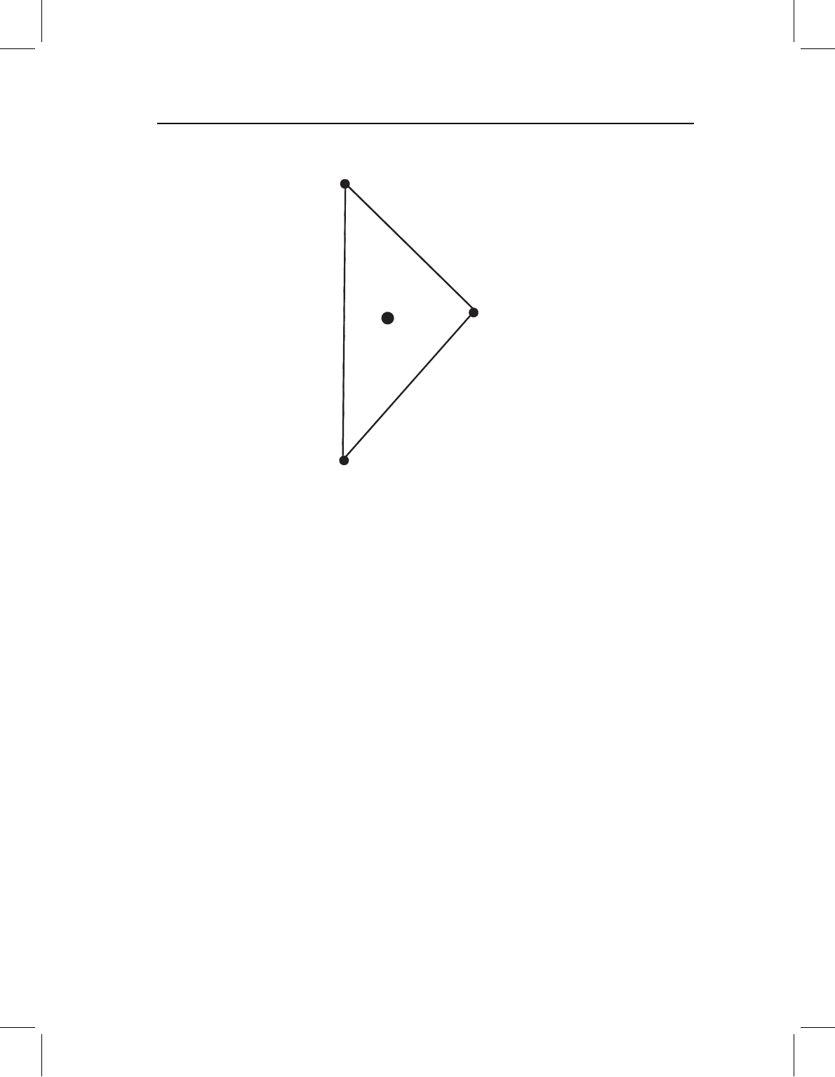
d. The centroid is located at (0.2333, −0.2333), or X =0.2333, Y =−0.233.

The centroid position is calculated:

(0 +0 +0.7)

= 0.2333

(−1 +0.5 −0.2)

=−0.2333

Figure 4.20 shows the location of the centroid.

(

0, ⫺1

)

(0, 0.5)

(0.7, ⫺0.2)

Figure 4.19 Answer to Exercise 4.1b.

chap-04 4/6/2004 17: 22 page 102

102 GEOMETRIC MORPHOMETRICS FOR BIOLOGISTS

(0, ⫺1)

(0, 0.5)

(0.7, ⫺0.2)

Figure 4.20 Answer to Exercise 4.1d.

e. We simply subtract the X-coordinate of the centroid (0.2333) from the first column

of A, and subtract the Y-coordinate of the centroid (−0.2333) from the second

column. This leaves us with:





−0.2333 −0.7667

−0.2333 0.7333

0.4667 0.0333





Note that if you add up the values in the first column you get zero, which is also

true for the second column. Thus the centroid position of the centered matrix is

(0, 0).

f. The centroid size is 1.2055. The centroid size is the square root of the summed

squared distances of the landmarks from the centroid, which is:

CS ={(0 −0.2333)

+(−1 −(−0.2333))

+(0 −0.2333)

+(0.5 −(−0.2333))

+(0.7 −0.2333)

+(−0.2 −(−0.2333))

}

= 1.2055

An easier approach is to use the centered form of the configuration matrix (with

the centroid set to zero). With this form, we can take the square root of the summed

chap-04 4/6/2004 17: 22 page 103

THEORY OF SHAPE 103

squared coordinates of the landmarks:

CS ={(−0.2333)

+(−0.7667)

+(−0.2333)

+ (0.7333)

+(0.4667)

+(0.0333)

}

= 1.2055

g. The resulting pre-shape space configuration is

pre-shape







−0.1936 −0.0630

−0.1936 0.6083

0.3871 0.0277







Note that the entries are identical to the centered matrix values (see (e) above)

divided by 1.2055.

2. Looking at the configuration:

a. There are four landmarks.

b. The configuration matrix is:







0.3 −1.0

0.25 −0.4

0.00.75

−0.20.35







c. The centroid is located at X

=0.0875, Y

=−0.075.

d. The centroid size CS =1.4087.

3. No! This might be K =6 and M =2 (a two-dimensional system), or K =4, M =3(a

three-dimensional system). If the data are in a row format, you cannot tell the value

of K or M from looking at it.

4. Looking at the configuration matrix:

a. The pre-shape space form of X is







0.7013 0.2550

−0.6376 −0.1275

−0.0638 −0.1275







b. The triangles can be iteratively rotated, or Equation 4.13 can be used:

θ = arctangent





j=1

−X



j=1



(4.13)

chap-04 4/6/2004 17: 22 page 104

104 GEOMETRIC MORPHOMETRICS FOR BIOLOGISTS

Substituting the appropriate values of X and Y for the reference (R) and target

(T) yields:

θ = tan

−1

{(0.1961 ×0.7013 +(−0.0981) × (−0.6376) +(−0.0981)

× (−0.0638) + (−0.6864) × 0.2550 +(−0.6864) × (−0.1275)

+ 0 × (−0.1275))/(0.6864 × 0.7013 +(−0.6864) × (−0.6376)

+ 0 × (0.0638) + 0.1961 × 0.2550 + (−0.0981) × (−0.1275)

+ (−0.0981) × (−0.1275))}

θ =−0.0562 radians =−3.2175

◦

5. Looking at the matrices:

a. To find the partial Procrustes distance between the two, we take the square root

of the summed squared differences in the landmark coordinates:

={(0.7146 −0.6864)

+(0.2150 −0.1962)

+ (−0.6438 −(−0.6864))

+(−0.0913 −(−0.0981))

+ (−0.0709 −0)

+(−0.1237 −(−0.0981))

}

=0.0933

b. Because ρ =2 arcsin(D

), ρ =2 arcsin(0.0933/2) =0.0933 radians; the two are

equal through three decimal places.

c. D

= sin(ρ), so D

=sin(0.0933) =0.0932.

References

Bookstein, F. L. (1996). Combining the tools of geometric morphometrics. In Advances in

Morphometrics (L. F. Marcus, M. Corti, A. Loy et al., eds) pp. 131–151. Plenum Press.

Dryden, I. L. and Mardia, K. V. (1998). Statistical Shape Analysis. John Wiley & Sons.

Fink, W. L. and Zelditch, M. L. (1995). Phylogenetic analysis of ontogenetic shape transformations:

a reassessment of the piranha genus Pygocentrus (Teleostei). Systematic Biology, 44, 343–360.

Kendall, D. (1977). The diffusion of shape. Advances in Applied Probability, 9, 428–430.

Marcus, L. F., Hingst-Zaher, E. and Zaher, H. (2000). Applications of landmark morphometrics to

skulls representing the orders of living mammals. Hystrix (n.s.), 11, 24–48.

Rohlf, F. J. (1998). On applications of geometric morphometrics to studies of ontogeny and

phylogeny. Systematic Biology, 47, 147–158.

Rohlf, F. J. (2000). On the use of shape spaces to compare morphometric methods. Hystrix (n.s.),

11, 8–24.

Slice, D. E. (2001). Landmark coordinates aligned by Procrustes analysis do not lie in Kendall’s

shape space. Systematic Biology, 50, 141–149.

Small, C. G. (1996). The Statistical Theory of Shape. Springer.

Zelditch, M. L., Bookstein, F. L. and Lundrigan, B. L. (1992). Ontogeny of integrated skull growth

in the cotton rat Sigmodon fulviventer. Evolution, 46, 1164–1180.

Zelditch, M. L., Fink, W. L., Swiderski, D. L. and Lundrigan, B. L. (1998). On applications of

geometric morphometrics to studies of ontogeny and phylogeny: a reply to Rohlf. Systematic

Biology, 47, 159–167.

chap-05 4/6/2004 17: 23 page 105

Superimposition methods

In Chapter 3 we presented a simple method for obtaining shape variables: the two-point

registration that produces Bookstein’s shape coordinates. We began with this method

because it is especially easy to understand, even without knowing any of the theory devel-

oped in Chapter 4. Having covered that theory, we now can develop a more general

approach to the problem of matching up shapes prior to comparison. This matching is

termed “superimposition” because the landmark configurations are placed on top of each

other (by the mathematical operations that do not alter shape, i.e. translation, scaling, and

rotation). Several superimposition methods are available; they differ in how these opera-

tions are applied. The objective of this chapter is to explain some of these superimposition

methods, compare them, and discuss their relative advantages and disadvantages. We also

discuss in some detail the issue of interpreting the pictures of superimposed landmarks. At

first sight different methods may appear to suggest different interpretations of the shape

differences, but to a large extent the differences are illusory – the pictures might look

different, but they have the same meaning.

Before discussing the alternative methods of superimposition, we first explain why we

would even want an alternative to Bookstein’s shape coordinates (BC). We then describe

a superimposition method that is based on a very similar approach. This method, called

sliding baseline registration (SBR), also involves a two-point registration, but the two

points are not entirely fixed (they are allowed to “slide” along one axis). Next, we present

the most widely used method, Procrustes generalized least squares (GLS), followed by

an alternative that is similar to it in some respects (variously called Procrustes resistant

fit, or resistant fit theta-rho analysis, RFTRA). After presenting all of these methods, we

summarize their similarities and differences, discuss the interpretation of their graphical

results, and conclude with recommendations regarding their uses.

Why we want an alternative to Bookstein shape coordinates

Recall that Bookstein’s shape coordinates (BC) are obtained by the two-point registration

method (Chapter 3). This procedure fixes the coordinates of two points at (0, 0) and (1, 0);

ISBN 0–12–77846–08 All rights of reproduction in any form reserved

chap-05 4/6/2004 17: 23 page 106

106 GEOMETRIC MORPHOMETRICS FOR BIOLOGISTS

thus the segment bounded by these landmarks (the baseline) has a standard orientation

and length in all specimens, and the coordinates of all the other landmarks indicate their

positions relative to the baseline. Fixing the baseline coordinates is the source of the prin-

cipal advantages of this superimposition method, and also of the main disadvantages. The

severity of the disadvantages may persuade you to use one of the other methods, even if

the purposes of those methods seem a bit obscure at first.

The most notable advantages of BC arise from standardizing the coordinates of the

baseline. Because four coordinates are fixed (X- and Y-coordinates of the two baseline

points), the number of variable coordinates is 2K −4 (where K is the number of landmarks).

Consequently, the number of variable coordinates is exactly the same as the number of

dimensions of the shape space they occupy, which is also the number of statistical degrees

(A)

(B)

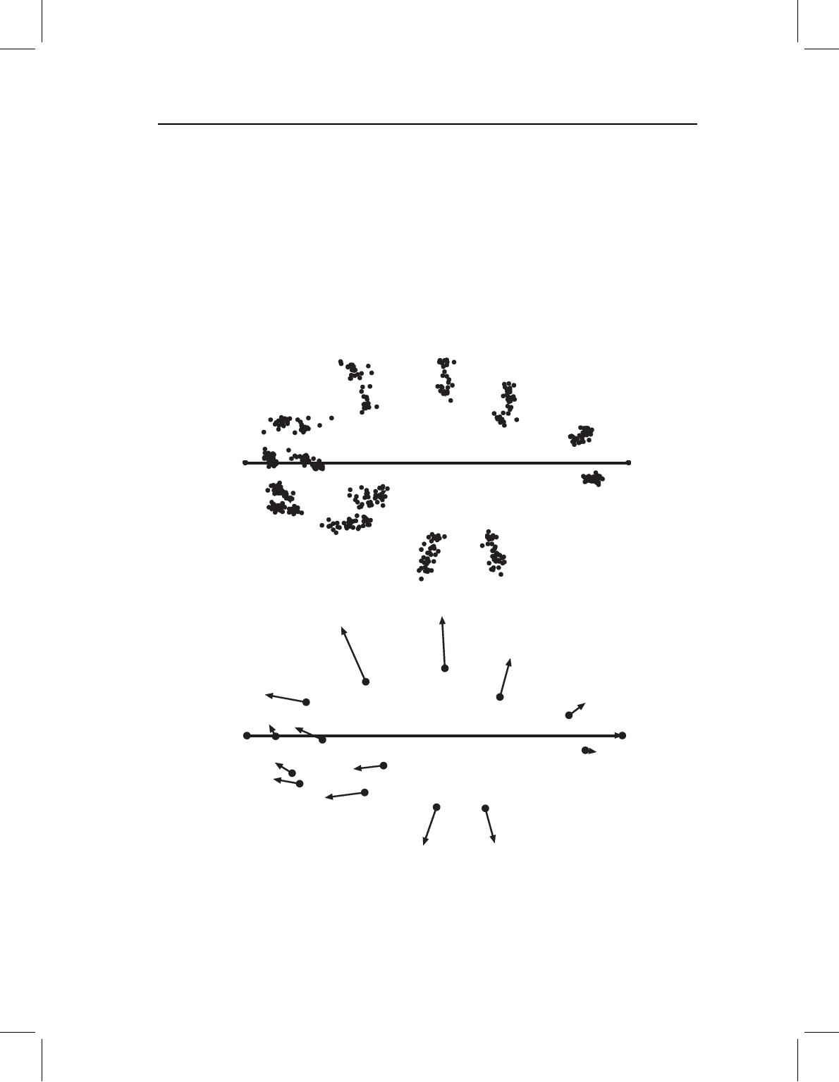
Figure 5.1 Variation in landmark positions relative to a fixed baseline for an ontogenetic series

of the piranha Serrasalmus gouldingi: (A) coordinates of landmarks relative to a fixed baseline that

extends between landmarks 1 and 7 (the tip of the snout and posterior termination of the hypural

bones); (B) vectors indicating displacements of landmarks relative to the fixed baseline. (The summed

squared lengths of these vectors does not equal the Procrustes distance between juvenile and adult

shapes.)

chap-05 4/6/2004 17: 23 page 107

SUPERIMPOSITION METHODS 107

of freedom. The advantage of the correspondence of these numbers is that we can perform

analytic tests like Hotelling’s T

without discarding variables. Because the four coordinates

of the baseline are fixed, the orientation of the baseline is standardized. The advantage of

this is that the pictures of the superimposed configurations are often quite easy to interpret,

especially if the baseline is an important morphological feature like an anatomical axis.

The most notable disadvantages of BC also lie in standardizing the coordinates of the

baseline. One of these disadvantages arises because there are no truly invariant landmarks;

every landmark varies in location relative to all of the others. Fixing the locations of the

two landmarks that serve as endpoints of the baseline means that the variance of those

landmarks must be put somewhere. In an ontogenetic series of the piranha Serrasalmus

gouldingi, superimposed at two landmarks near the dorsoventral midline (Figure 5.1A),

we can see that the three most dorsal landmarks vary primarily along the dorsoventral axis.

When we regress these coordinates on log centroid size (using methods discussed in Chapter

10), we see that these landmarks move away from the midline during growth (Figure 5.1B).

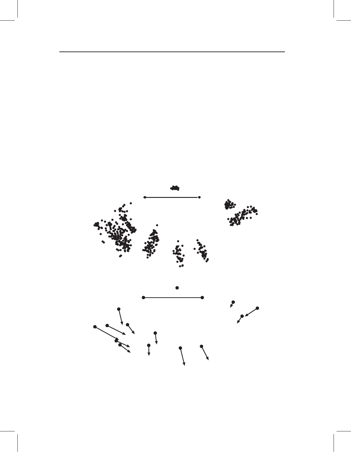
If two of the dorsal landmarks are used as the baseline, the pictures look strikingly

different (Figure 5.2). The dorsoventral component has been removed from all three dorsal

(A)

(B)

Figure 5.2 Ontogenetic variation in S. gouldingi visualized relative to a baseline on the dorsal body

(landmarks 3 and 5): (A) coordinates of landmarks relative to the baseline; (B) vectors indicating

displacements of landmarks relative to the fixed baseline. (Note the greater apparent magnitude of

the variance landmarks compared to Figure 5.1.)