Teodorescu P.P. Mechanical Systems, Classical Models Volume I: Particle Mechanics

MECHANICAL SYSTEMS, CLASSICAL MODELS

522

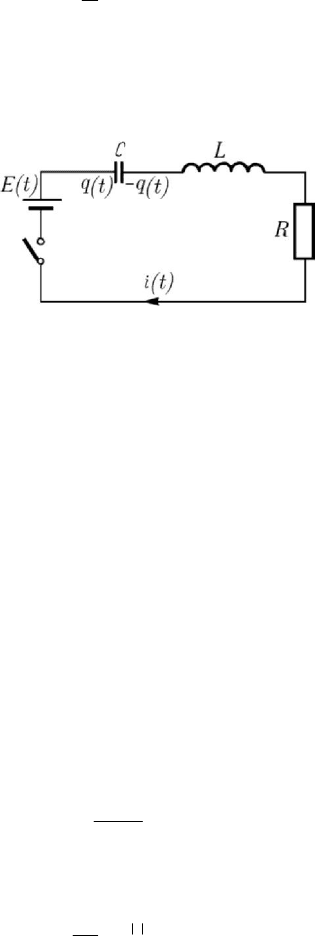
() () () ()Lqt Rqt qt Et

++ = 

, 0t > ,

(8.2.58)

corresponding to Kirchhoff’s second law. Cauchy’s problem for this circuit consists in

the determination of the function

()qt which satisfies the equation (8.2.58) for 0t >

and the initial conditions

Figure 8.49. Electro-mechanical analogy.

(0)qq

(0)qi

 ,

(8.2.58')

where

q and

i are the charge and the intensity of the current at the moment 0t = ,

respectively. The correspondence

Lm→ , Rk

′

→ , 1/Ck→ , () ()Et Ft→ ,

() ()qt xt→ , () ()it xt→  leads to an interesting electro-mechanical analogy, which

allows an experimental determination of the corresponding mechanical quantities.

2.2.11 Case of an arbitrary perturbing force

We consider first of all the non-damped motion with arbitrary perturbing forces,

governed by an equation of the form (8.2.42), in case of elastic forces of attraction, or

of the form

()xxftω−=

(8.2.59)

in case of repulsive elastic forces. The fundamental solution of the operator

22 2

Dd/dt ω=+ is

sin

() ()

Et t

= , 0ω > ,

(8.2.60)

where

()tθ is Heaviside’s distribution. As well, the distribution of function type

() e

−

=− , 0ω > ,

(8.2.61)

is the fundamental solution of the operator

22 2

Dd/dt ω=−; this distribution is

generated by a continuous and everywhere differentiable function, excepting the origin.

Using the considerations in App., Subsec. 3.3.1, we may write

D() ()

Et tδ= ,

Dynamics of the particle in a field of elastic forces

523

1, 2i =

, where ()tδ is Dirac’s distribution. If to the particular fundamental solution

()Et, the support of which is the real axis, we add the solution e/2

tω

ω , 0ω > ,

corresponding to the homogeneous equation, then we find the fundamental solution

sinh

() ()

Et t

= ,

0ω >

(8.2.61')

the support of which belongs to the interval

[0, )

∞

; hence

D() ()Et tδ= . Denoting

generically by

()Et

the fundamental solution corresponding to one of the two cases,

we may write – for an arbitrary load

()

t – the solution

() () ()xt E t ft

∗ ,

(8.2.62)

in distributions, where we have introduced the convolution product. If

()

t is an

integrable function, it results

() () ( )d () (, )dxt ftE t ftGtττ ττ

+∞ +∞

−∞ −∞

=−=

∫∫

, 0t ≥ ,

(8.2.62')

where

(, )Gtτ is Green’s function corresponding to one of the equations (8.2.42),

(8.2.59).

Let us put initial conditions of the form

lim ( )

xt x

→+

lim ( )

xt v

→+

 ,

(8.2.63)

in case of a problem of Cauchy type. By a prolongation with zero for

0t <

, we

introduce the functions

() ()()xt txtθ= , () () ()

ttftθ= ;

(8.2.64)

in this case, the equation (8.2.42), which is written for

0t ≥ , is of the form

() () ()

xt xt f t

ω+=



where the sign “tilde” corresponds to the differentiation in the usual sense. Using the

formula (1.1.50), we notice that

() () ()

xt xt x t

δ=+



() () () ()

xt xt v t x t

δδ=++





so that one obtains

() () () () () ()xt xt f t v t x t qtωδδ+=++=





(8.2.65)

MECHANICAL SYSTEMS, CLASSICAL MODELS

524

in distributions, where the differentiation takes place in the sense of the theory of

distributions. The formula (8.2.62) allows to write

() ()sin () () ()xt t t f t v t x tθω δ δ

=∗++

⎡

⎤

⎣

⎦



where we took into account (8.2.60). Effecting the convolution products, it results

() ()sin () ()cos ()sin

xt t t f t x t t t tθω θ ωθω

ωω

=∗++

(8.2.65')

while, if

()

t is a locally integrable function, then we get

() cos sin ( )sin ( )d

xt x t t f tωω τωττ

ωω

=++ −

∫

, 0t ≥ ;

(8.2.65'')

the integral which intervenes is known as the Duhamel integral. If the perturbing force

is a shock at the initial moment, then we have

() ()

tftδ

(8.2.66)

where

is a quantity the dimension of which is that of a velocity (dimensionally

[

]

() Ttδ

−

= ); we obtain

() ()cos ()sin

xt x t t t tθω θω

=+ .

(8.2.66')

We thus notice that the apparition of a shock at the initial moment is equivalent to the

introduction of a supplementary initial velocity.

Considering the same problem for the equation (8.2.59), written in the form

() () ()xt xt qtω−=



(8.2.67)

it results, analogously,

() ()sinh () ()cosh ()sinh

xt t t f t x t t t tθω θ ωθω

ωω

=∗++

;

(8.2.67')

()

t is a locally integrable function, then we get

( ) cosh sinh ( )sinh ( )d

xt x t t f tωωτωττ

ωω

=++ −

∫

0t ≥

(8.2.67'')

As well, in case of a perturbing force of the form (8.2.66), we have

() ()cosh ()sinh

xt x t t t tθω θω

=+ ,

(8.2.66'')

Dynamics of the particle in a field of elastic forces

525

and we obtain a result analogous to that above.

In case of a bilocal problem, we put conditions of the form

()xt x

(8.2.68)

assuming that

[

]

,ttt∈ . In case of Cauchy type conditions for

, we may write

11 1

() cos ( ) sin ( ) ( )sin ( )d

xt x t t t t f tωω τωττ

ωω

=−+−+ −

∫

considering an elastic force of attraction and assuming that

()

t is a locally integrable

function. The second bilocal condition (8.2.68) leads to

2 1 21 21 2

cos ( ) sin ( ) ( )sin ( )d

xx tt tt f tωω τωττ

ωω

=−+−+ −

∫

so that we can determine the velocity

v at the initial moment; eliminating this velocity

between the last two relations, one obtains the solution of the bilocal problem in the

form

{

() sin ( ) ( )sin ( )d

sin ( )

xt t t f t

ωτωττ

ωω

=−−

−

∫

[

1212

sin ( ) ( )sin ( )d sin ( )

tt f t x t tωτωττωω−− −+ −

∫

]

}

sin ( )xttω+−

ttk

≠+

, k

∈

` .

(8.2.69)

In case of a repulsive elastic force, it results

{

( ) sinh ( ) ( )sinh ( )d

sinh ( )

xt t t f t

ωτωττ

ωω

=−−

−

∫

[

1212

sinh ( ) ( )sinh ( )d sinh ( )

tt f t x t tωτωττωω−− −+ −

∫

]

}

sinh ( )xttω+−

(8.2.69')

for the same bilocal problem.

In the general case of a law of motion of the form

()mx k x kx F t

′

+=  ,

(8.2.70)

where

k−∞ <

, k

′

<∞, which corresponds to all possibilities of motion previously

considered, we put Cauchy’s problem in the form (8.2.63). By a prolongation with zero

for

0t <

, of the form (8.2.64),

() () ()Ft tFtθ=

(8.2.64')

MECHANICAL SYSTEMS, CLASSICAL MODELS

526

and taking into account the connection between the derivatives in the usual sense and in

the sense of the theory of distributions for the regular distributions thus obtained, we

may write, as above, the corresponding equation in distributions

00 0

() () () () ( )() () ()mx t k x t kx t F t mv k x t mx t Q tδδ

′′

++=++ + =



 

(8.2.70')

which includes the initial conditions. The solution of this problem is given by

() () ()xt Et Qt

∗ ,

(8.2.71)

where

()Et is the fundamental solution in the sense of the theory of distributions,

which verifies the equation

() () () ()mE t k E t kE t tδ

′

++=

 

(8.2.71')

Applying the Laplace transform in distributions, we obtain

(

)

[

]

() 1mp k p k L E t

′

+=,

where

is the new variable in the space of transforms; it results

[]

L()

()()

mp p p p

mp k p k

−−

′

p αβ=− + ,

p αβ

−−,

′

= ,

′

⎛⎞

=−

⎜⎟

⎝⎠

Three cases of integration are thus put in evidence. If

4kkm

′

(8.2.72)

then we may write (

0β > , β

∈

\ )

[]

11 1

L()

mpp ppβ

⎛⎞

=−

⎜⎟

−−

⎝⎠

wherefrom

()

() e e ()e sinh

pt pt t

Et t t

θβ

ββ

−

=−= .

(8.2.72')

After effecting the convolution products, the solution (8.2.71) takes the form

000

( ) ( )e sinh ( ) ( )e cosh ( )sinh

xt t t Ft t x t v x t

αα

θβθ βαβ

ββ

−−

⎡

⎤

=∗+ ++

⎢

⎥

⎣

⎦

;

(8.2.73)

Dynamics of the particle in a field of elastic forces

527

()Ft is a locally integrable function, then we can write

000

() e cosh ( )sinh

xt x t v x t

βαβ

−

⎡⎤

=++

⎢⎥

⎣⎦

()esinhd

ατ

τβττ

−

+−

∫

, 0t ≥ .

(8.2.73')

′

> , then we denote 0αλ

> (viscous damping), while if 0k

′

< , then we

denote

0αλ

−< (self-sustained oscillations). If 0k > (elastic forces of attraction),

then we denote

/km ω=

, βω

′

(

λω> ), while if 0k

(repulsive elastic

forces), then we denote

/km ω−=, βω

. We pass thus to the notation previously

used.

4kkm

′

(8.2.74)

and

0β < ,

β ∈ ^

, iβω

′

ωωλ

′

⎛⎞

′

=− = −

⎜⎟

⎝⎠

then we may write (one can have only

0k > , hence elastic forces of attraction)

() ()e sin

Et t t

θω

−

′

;

(8.2.74')

the solution of Cauchy’s problem is

000

() ()e sin () ()e cos ( )sin

xt t t Ft t x t v x t

αα

θωθ ω αω

ωω

−−

⎡

⎤

′

′′

=∗+++

⎢

⎥

′′

⎣

⎦

(8.2.75)

and, in the case in which

()Ft is a locally integrable function, we obtain

000

() e cos ( )sin

xt x t v x t

ωαω

−

⎡⎤

′

=++

⎢⎥

′

⎣⎦

()esind

ατ

τωττ

−

′

+−

′

∫

, 0t ≥ .

(8.2.75')

4kkm

′

(8.2.76)

then we have

0β = , so that

[

]

L() 1/( )Et mp α=+; the fundamental solution is

() ()e

Et tt

−

= .

(8.2.76')

MECHANICAL SYSTEMS, CLASSICAL MODELS

528

The solution of the boundary value problem reads

[]

00 0

() ()e () ()e ( )

xt tt Ft t x v x t

αα

θθ α

−−

=∗+ ++,

(8.2.77)

while if

()Ft is a locally integrable function, then we get

[]

00 0

() e ( ) ( )e d

xt x v x t Ft

αατ

ατττ

−−

=+++ −

∫

0t ≥

(8.2.77')

According to the above relations, for the last two cases we obtain a viscous damping or

self-sustained oscillations for

αλ

± , respectively.

In the particular case of homogeneous initial conditions (

0xv

= ) we remain

only with the first terms of the formulae (8.2.73), (8.2.75) and (8.2.77).

The vibratory phenomena considered above, for which the parameters

,,mkk

′

are

constant, are – in general – in permanent régime. Such phenomena may be due, for

instance, to a perturbing force, which is applied at the initial moment and remains

constant in time, of the form

() ()Ft F tθ= ;

(8.2.78)

we obtain thus

[]

e ( sinh cosh ) for 4 ,

( ) 1 (1 )e for 4 ,

e ( sin cos ) for 4 ,

tt kkm

xt t k km

tt kkm

αββ ββ

αωωω ω

−

⎧

′

−+−>

⎪

′

=−+ =

⎨

⎪

′

−+−<

⎪

⎩

(8.2.78')

for

0t ≥ . Passing from a permanent régime to another one, a transitory phenomenon

takes place; for instance, the transitory phenomena appear by the introduction or by the

elimination of a perturbing force, as well as – in general – by any variation of the

parameters of the considered phenomena. E.g., in case of a shock at the initial moment,

given by

() ()Ft F tδ

(8.2.79)

we obtain

e sinh for 4 ,

( ) e for 4 ,

e sin for 4 ,

tkkm

xt t k km

tkkm

−

⎧

′

⎪

′

⎨

⎪

′′

⎪

′

⎩

(8.2.79')

Dynamics of the particle in a field of elastic forces

529

for

0t ≥ ; this result corresponds to the fundamental solutions (8.2.72'), (8.2.76') and

(8.2.74'), as well as to the velocity which appears in the previously considered case (it is

obtained by differentiating the formula (8.2.78') with respect to time).

2.2.12 Oscillations with variable characteristics

The oscillations with variable characteristics (parametric oscillations) are the

oscillations of a mechanical system the parameters of which (mass, frequency,

dimensions, elastic coefficient, damping coefficient etc.) are functions of time. In the

absence of a perturbing force, the mathematical model of such a mechanical

phenomenon leads to a differential equation of the form

() () 0xtxtxαβ

+=  ,

(8.2.80)

where

()tα and ()tβ are periodic functions. By the substitution

(1/2) ( )d

() ()e

xt ut

α−

∫

we obtain the equation

() 0utuγ+= ,

() () () ()

tt t tγβ α α=− − .

(8.2.81)

To deduce the aspect of the solution or to find an approximate solution of this

equation may be a different task from case to case. The general solution can be written

in the form

() e () e ()

ut t t

λμ

ϕψ=+,

(8.2.81')

where the coefficients

λ and μ are characteristic coefficients of the equation, while

()tϕ and ()tψ are periodic functions of period T (as well as the function ()tγ ),

which have to be determined. One may put the condition

()()ut T kut

= ,

(8.2.81'')

where

(, )kkλμ

. Thus, if we know the motion during a period, then the motion in

the following period is obtained by multiplying the elongation of the first period by the

factor

k a.s.o. If 1k < , then the elongations tend to zero and the oscillations are

damped; if

1k > , then the elongations increase in time and the motion becomes

instable.

For instance, in case of a mathematical pendulum of variable length

()llt= , the

equation of motion which specifies the generalized co-ordinate

()tθθ

()

sin 0

lgl

θθ



;

(8.2.82)

MECHANICAL SYSTEMS, CLASSICAL MODELS

530

in case of small oscillations, we obtain the equation

()

() ()

lt lt

θθθ++=



 

(8.2.82')

2.2.13 Non-linear oscillations

We say that a mechanical system represents a non-linear oscillatory system if, in the

differential equation of motion, one or several characteristic parameters (mass, elastic

coefficient, frequency etc.) depend on the displacement

x . In general, the differential

equation of these oscillations is of the form

(,;) 0xfxxt

=  ,

(8.2.83)

resulting from Newton’s equation (which puts in evidence the linkage between the

elastic force and the displacement) or, in particular, of the form

(,) 0xfxx

=  ,

(8.2.83')

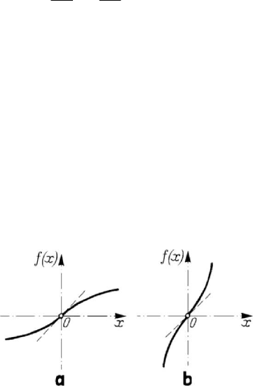
Figure 8.50. Non-linear vibrations determined by the equation () 0xfx



; diagrams

()fx vs

for

0x >

: case () 0fx

′

(a); case () 0fx

′

> (b).

as the non-linear vibration is non-autonomous or autonomous, respectively. If the non-

linear term depends only on

x , then the function ()

x which intervenes is called arc

characteristic; the most times, in practice, the graphic of the function

()

x is

symmetric with respect to the origin (

()

x is an odd function, that is ()

x−

()

x=− ). If the graphic of the function ()

x has the concavity towards down in the

vicinity of the origin for

0x > , hence if () 0

′

(Fig.8.50,a), then the arc

characteristic is weak, while if, in the same vicinity, the graphic of the function

()

has the concavity towards up for

0x > , hence if () 0

′

(Fig.8.50,b), then the arc

characteristic is strong.

In case of great oscillations of the simple pendulum, the non-linear character of the

phenomenon is put into evidence in the equation (7.1.38'). Developing

sin θ into a

power series, we obtain, in a first approximation, the linear differential equation

(7.1.45). In a second approximation (non-linear approximation, in which we take two

terms in the series development), we may write

Dynamics of the particle in a field of elastic forces

531

θωθ

⎛⎞

−=

⎜⎟

⎝⎠



;

(8.2.84)

in this case,

(

)

() /6

θωθθ=− and

() 0

θωθ

′′

−< for 0θ > , the arc

characteristic being thus weak.

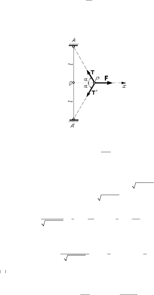
Figure 8.51. Motion of a particle situated at the middle of an elastic thread.

Let us consider also the case of a particle

P of mass m , situated at the middle of an

elastic thread fixed at the points

A and A

′

, 2AA l

′

(e.g., the case of a training ball

for boxing); in the position

O of stable equilibrium, the tension in the thread is

T (we

suppose that the thread is tensioned). Perturbing the position of equilibrium by a

displacement normal to

′

, the particle reaches the position P (Fig.8.51), being

acted by the tensions

T and

′

T ,

(

)

TTTkl x l

′

=+ +−, and by the

perturbing force

F ,

2cos 2 /FT Txlxα== +. Observing that

1/2

11 1

−

⎛⎞ ⎛ ⎞

=+ ≅−

⎜⎟ ⎜ ⎟

⎝⎠ ⎝ ⎠

we obtain

(

)

2( )

22()

Tklx

Fkx T klT

−

=+ ≅ +−

;

xl , then we remain only with the first term (the case of a linear elastic force). In

the non-linear case considered (the second approximation), the equation of motion is

20xx xαβ

+= ,

> ,

kl T

−

> ,

(8.2.85)

Teodorescu P.P. Mechanical Systems, Classical Models Volume I: Particle Mechanics

Подождите немного. Документ загружается.