Teodorescu P.P. Mechanical Systems, Classical Models Volume I: Particle Mechanics
Подождите немного. Документ загружается.

MECHANICAL SYSTEMS, CLASSICAL MODELS
512
If
00
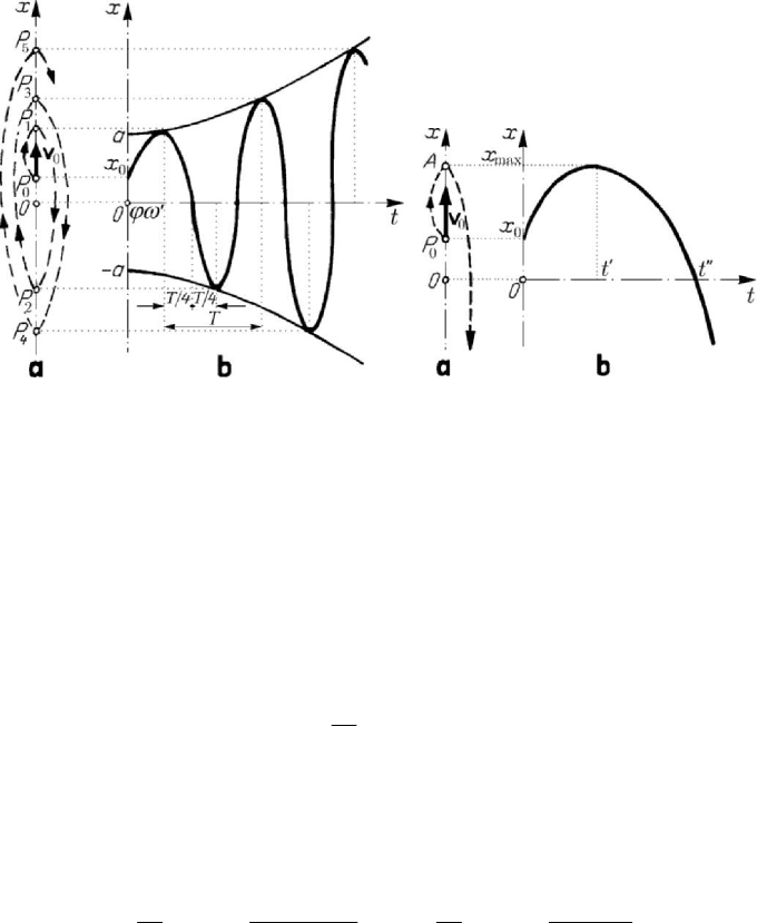
0 vxλ<< , then the particle starts from
0
P , reaches A at the moment
000
/( )tv xvλλ
′
=− and then changes of direction and tends to infinity in the
negative direction of the
Ox -axis (Fig.8.39,a); the diagram of motion has a maximum
for
tt
′
=
and pierces the Ot -axis at
000
/( )tx xvλ
′
′
=
− (Fig.8.39,b). If
00
vxλ≥ ,
Figure 8.38. Self-sustained motion of a particle; Figure 8.39. Self-sustained motion of a
subcritical damping. Trajectory (a); particle; critical damping, case
diagram
()xt vs t (b).
00
0 vxλ
<
< : trajectory (a);
diagram
()xt vs t (b).
then the particle starts from
0
P and tends to infinity in the positive direction of the Ox -
axis (Fig.8.35,a), the diagram of motion being that of Fig.8.35,b. If
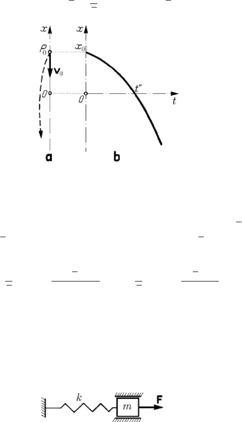
0
0v ≤ , then the
particle tends to infinity in the negative direction of the
Ox -axis (Fig.8.40,a), while the
diagram of motion pierces the
Ot -axis at tt
′
′
=
(Fig.8.40,b). Analogously, for ωλ<
(supercritical damping,
1χ > ) we obtain
000
1
() e cosh ( )sinh
t
xt x t v x t
λ
ωλω
ω
⎡⎤
′
′′′
=+−
⎢⎥
′′
⎣⎦
,
(8.2.39''')
the pseudopulsation ω
′′
being given by (8.2.17). In what concerns the trajectory and
the diagram of motion, we obtain the same qualitative results as
00
0()vxλω
′′
<
<− ,
as
00
()vxλω
′′
≥− or as
0
0v
≤
, respectively (Figs 8.39, 8.35, 8.40); in this case
0
2
00
1
arg tanh
v
t
xv
ω
ω
ωλ
′
′
′
=
′′
−
,
0
00
1
arg tanh
x
t
xv
ω
ωλ
′
′
′′
=
′′
−
.
If the elastic force is repulsive, then the equation of motion has the form
2
20xxxλω
−
−= ,
(8.2.40)
Dynamics of the particle in a field of elastic forces
513
and we are led to
000
1
() e cosh ( )sinh
t
xt x t v x t
λ
ωλω
ω
⎡⎤
=+−
⎢⎥
⎣⎦
,
(8.2.40')
Figure 8.40. Self-sustained motion of a particle; critical damping, case
0
0v ≤ :
trajectory (a); diagram
()xt
vs t (b).
with the same initial conditions and the notation (8.2.18'''). The trajectory and the
diagram of motion are qualitatively given for
0
0v ≥
and for
00
()vxωλ
=
−− in
Fig.8.35, for
00
() 0xvωλ−− < < in Fig.8.36 and for
00
()vxωλ
<
−− in Fig.8.40;
we notice that
0
2
00
1
arg tanh
v
t
vx
ω
ω
λω
−
′
=
+
,
0
00
1
arg tanh
x
t
xv
ω
ωλ
′′
=
−
.
2.2.8 Influence of perturbing forces. Resonance
The intervention of a perturbing force
F
leads to a forced motion (a constraint or
forced oscillation) of a particle
P
, unlike the free motion (free oscillation) considered
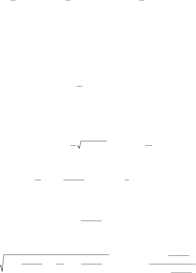
till now. The most simple physical model of a mechanical system with a simple degree
of freedom acted upon by such a force is that of a non-damped forced linear oscillator,
represented in Fig.8.41.
Figure 8.41. Model of a non-damped forced linear oscillator.
Let us consider firstly the case of a periodic force
()FFt
=
, which fulfils the
Lejeune-Dirichlet sufficient conditions, that is which is developable into a Fourier
series
0
11
( ) cos sin ... cos sin ...
nn
F t pt pt npt nptαα α α α
′′′ ′ ′′
=+ + ++ + +,
(8.2.41)
MECHANICAL SYSTEMS, CLASSICAL MODELS
514
where
0
1
()d
T
Ft t
T
α =
∫
,
2
()cos d
n
T
Ft npt t
T
α
′
=
∫
,
2
()sin d
n
T
Ft npt t
T
α
′′
=
∫
,
(8.2.41')
the period
2/Tpπ= on which is effected the integration may begin from a point
arbitrarily chosen. In case of a non-damped linear oscillator subjected to a perturbing
force, the equation of motion is of the form
2
()xxftω+= ,
(8.2.42)
where we use the previous notation and where
1
() ()
f
tFt
m
=
.
(8.2.43)
We notice that the term
0
α in the expansion into a series leads only to a change of
origin for
()xt , so that it may be neglected. For each term of the Fourier series one
obtains a particular integral of the same type, leading to the corresponding motion; it is
thus sufficient to consider the influence of only one term of the form
cos( )ptαϕ− ,
22
111
1
m
αα α α
′
′′
== +
,
arctan
α
ϕ
α
′
′
=
′
.
(8.2.44)
For
() cos( )
f
tptαϕ=−, we find
0
0
22
( ) cos sin cos cos sin sin cos( )
v
p
xt x t t t t pt
p
α
ωω ϕωϕω ϕ
ωω
ω
⎡
⎤
=+− + −−
⎣
⎦
−
,
(8.2.42')
with the initial conditions (8.2.23'); we may also write
22
() cos( ) cos( )xt a t pt
p
α
ωψ ϕ
ω
=−+ −
−
,
(8.2.42'')
where
22
00
22 2 22
cos sin
1
p
ax v
pp
αϕ α ϕ
ωωω
⎛⎞⎛⎞
=− + −
⎜⎟⎜⎟
−−
⎝⎠⎝⎠
,
0
22
0
22
sin
arctan
cos
p
v
p
x
p
αϕ
ω
ψ
αϕ
ω
ω
−
−
=
⎛⎞
−
⎜⎟
−
⎝⎠
.
(8.2.42''')
One observes thus that the motion of the particle may be obtained as an interference of
two harmonic vibrations: the proper vibration (the proper oscillation) of pulsation
ω
Dynamics of the particle in a field of elastic forces
515
and the forced vibration (the forced oscillation) of pulsation
p , as it was shown in
Subsec. 2.2.4. If, in particular, we assume homogeneous initial conditions
(
00
0xv==) and if the phase shift of the perturbing force vanishes ( 0ϕ = ), then it
results
22
() (cos cos )xt pt t
p
α
ω
ω
=−
−
.
(8.2.45)
If the pulsation
p
differs much from the pulsation ω (p ω or p ω ), then the
diagram of motion is that in Fig.8.22 (the case
p ω , hence a proper vibration of
great pulsation “carried” by a forced vibration of small pulsation); we notice that the
maximal elongation of the resultant motion is practically equal to the double of the
amplitude of one of the motions (
(
)
22
max
2/xpαω≅−). If the two pulsations are
close in magnitude, then one obtains the phenomenon of “beats” (Fig.8.23).
If
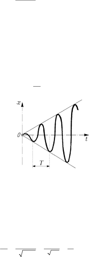
p ω= , then it results a non-determination in (8.2.45), as well as in (8.2.42'). If
p ω→
, then one obtains at the limit (we use L’Hospital’s theorem)
() sin
2
xt t t
α
ω
ω
= ,
(8.2.46)
Figure 8.42. Phenomenon of resonance. Diagram ()xt vs
t
.
for the law of motion (8.2.45). In case of the equation of motion (8.2.42') we get an
analogous result (supplementary harmonic vibrations are added). The diagram of
motion (8.2.46) is a sinusoid of amplitude modulated along the straight lines
/2xtαω=± and of pseudoperiod 2/T πω
=
(Fig.8.42). The amplitude increases
very much, in arithmetic progression, and the phenomenon is called resonance, being
extremely dangerous for civil and industrial constructions or for engine building; the
increasing velocity of the amplitude is given by the slope
1
11
/
2
2
2/
c
Fm
FF
k
km
km
α
ω
===
′
,
(8.2.47)
hence it is in direct proportion to the amplitude
11
Fm mαα
=
= of the perturbing
force and in inverse proportion to the critical coefficient of damping (8.2.14). If

MECHANICAL SYSTEMS, CLASSICAL MODELS
516
2
st
11
//xFkFmω== is the static displacement produced by the force
1
F
(corresponding to the relation of proportionality between the elastic force and the
displacement), then we may express the amplitude
A of the forced vibration in the
form
st
Ax=
A
, A being an amplification factor of the forced vibration, given by
22 2
11
1/ 1p ωη
==
−−
A
,
(8.2.48)
where we have introduced the relative pulsation
p
η
ω
=
,
(8.2.48')
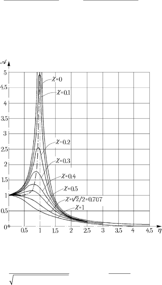
Figure 8.43. Phenomenon of resonance. Diagram A vs η .
which is a non-dimensional ratio. The diagram of the absolute value
A
is given in
Fig.8.43.
Figure 8.44. Model of a viscous damped forced linear motion.
If a viscous damping intervenes, then we use the physical model in Fig.8.44, being
led to the equation of motion
2
2cosxxx ptλω α++= ,
(8.2.49)
with the previously introduced notations (for the sake of simplicity, we assumed
0ϕ = ). To fix the ideas, we assume to be in the case of a subcritical damping ( 1χ < );
the motion of the particle is given by
Dynamics of the particle in a field of elastic forces
517
12
() e cos( ) cos sin
t
xt a t C pt C pt
ω
ωψ
′
−
′
=−++
,
(8.2.49')
where
(
)
()
22
1
2
22 22
4
p
C
pp
ωα
ωλ
−
=
−+
,
()
2
2
22 22
2
4
p
C
pp
λα
ωλ
=
−+
,
(8.2.49'')
the last two terms corresponding to the forced motion. Taking into account the
exponential term, the proper motion is rapidly damped, so that we may consider the
forced motion in the form
() cos( )xt A pt ϕ
=
− ,
(8.2.50)
Figure 8.45. Viscous damped forced linear motion. Diagram A vs η.
with
()
2
22 22
4
A
pp
α
ωλ
=
−+
,
22
2
arctan
p
p
λ
ϕ
ω
=
−
.
(8.2.50')
Using the notations introduced above and the damping factor (8.2.14'), we may also
write
MECHANICAL SYSTEMS, CLASSICAL MODELS
518
()
2
222
1
14ηχη
=
−+
A ,
2
2
arctan
1
χη
ϕ
η
=
−
.
(8.2.50'')
The diagram of the amplification factor
()η
=
A
A is given in Fig.8.45 for various
values of the damping factor
χ . We define a resonance in amplitude for the values
2
res
12 1ηη χ==−<, 1/ 2χ ≤ ,
(8.2.51)
for which the amplification factor has a maximum
max
2
11
2
21
χ
χχ
=>
−
A .
(8.2.51')
One observes that, in case of the phenomenon of resonance, the amplitude is as smaller
as the damping is greater, the diagram of the function being planished for a great
damping; the effect of damping appears especially in the vicinity of the resonance zone
(
1η ≅ ). If the damping is very small ( 1χ ), then the resonance in amplitude
appears for
1η ≅ , the amplification factor being given by
max
1/2χ≅
A
.
Eliminating
χ between (8.2.51) and (8.2.51'), we get
4
max res
1/ 1 η=−A , that one
being the locus of the points of maximum of the diagrams for various values of
χ
(represented by a dot-dash line). These points are at the left of the line
1η = ; on this
line one has
1/2χ=
A
.
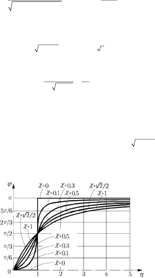
Figure 8.46. Viscous damped forced linear motion. Diagram ϕ vs η.
The diagram of the phase function
()ϕϕη
=
is given in Fig.8.46 for various values
of the coefficient
χ . We notice that, in case of a non-damped system, the phase is
0ϕ = , under the resonance ( 1η
<
), the vibration being in phase with the perturbing

Dynamics of the particle in a field of elastic forces
519
force, or
ϕπ= , over the resonance ( 1η > ), the vibration being in phase opposition
with respect to the perturbing force; in case of a damped system there exists always a
phase shift between the perturbing force and the vibration. For
1η
<
, as χ (hence, the
damping) increases, so the phase shift between the motion and the perturbing force
increases too, the motion remaining behind that force. For
1η > , as χ (hence, the
damping) increases, so the phase shift decreases, the motion remaining behind the
perturbing force too. For a very great
η , the phase shift increases no matter the
damping and the motion tends to be in opposition with the perturbing force. But the
opposition is obtained rigorously only in the absence of the damping (
0η = ). For
1η = one obtains /2ϕπ= for all the damping coefficients χ ; one may define thus a
phase resonance for which the vibration is in quadrature with the perturbing force.
Starting from the equation of motion
1
cosmx k x kx F pt
′
+
+=
(8.2.52)
and multiplying by
x , we get
2
1
d
() cos
d
TV kx Fx pt
t
′
+=− +
;
(8.2.53)
it is thus seen that the mechanical energy does not remain constant, because the second
member of this relation is – in general – non-zero. If we equate this member to zero,
assuming that
0x N , we find
1
0
sin
F
xx pt
kp
=+
′
;
(8.2.53')
hence, the amplitude of the motion is
1
/Fkp
′
, corresponding to the amplitude
resonance (
1/2χ=
A
for
1η
=
).
2.2.9 Mechanical impedance. Transmissibility
Using the complex representation in Subsec. 2.2.3, we can write the equation of
motion (8.2.52) in complex form
mz k z kz F
′
+
+= ,
(8.2.54)
where we denoted
i
0
e
pt
zz=
and
i
1
e
pt
FF=
; replacing
izpz
=
,
2
zpz=− , we may
write
FZz
=
, (8.2.55)
where we have introduced the mechanical impedance
2
iZkmp kp
′
=− + ,
(8.2.55')
MECHANICAL SYSTEMS, CLASSICAL MODELS
520
which is a constant of proportionality, extending thus the notion of elastic constant. For
an elastic spring, the impedance is
Zk
=
, for a mass m we may write
2
Zmp=− ,
while for a linear (viscous) damping it results
iZkp
′
=
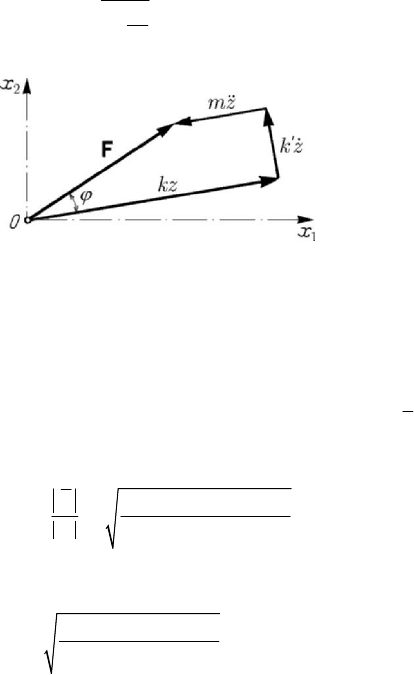
. We notice that the equation
(8.2.54) may be obtained as a sum of vectors in the complex plane (Fig.8.47).
Projecting on the direction of the force
F
and on a normal to it, one finds again the
amplitude
A and the phase shift ϕ given by (8.2.50'). Using the analogy with the
constants corresponding to elastic springs (see Subsec. 2.2.1) and the formulae (8.2.25),
(8.2.25'), we can express the impedance equivalent to
n impedances
i
Z
, 1,2,...,in= ,
linked in parallel, in the form
1
n
i
i
ZZ
=
=
∑
,
(8.2.56)
while for the impedance equivalent to the same impedances linked in series we may
write
1
1
1
n
i
i
Z
Z
=
=
∑
.
(8.2.56')
Figure 8.47. Viscous damped forced linear motion. Complex representation.
An examination of the physical model of a mechanical system constituted of an
elastic spring and a linear damper which act in parallel on a mass (Fig.8.44) leads to the
notion of transmissibility as the ratio
T
C between the amplitude of the force
()Ft kx kx
′
=+ transmitted to the fixed element and the amplitude of the perturbing
force
()Ft which acts upon the mass m . Introducing the impedance iZk kp
′
=+ ,
2
iZkmp kp
′
=− + , it results
()
222
2
222
T
Z
kkp
C
Z
kmp kp
′
+
==
′
−+
;
with the aid of the previous notations, we may also write
()
22
2
222
14
14
T
C
χη
ηχη
+
=
−+
.
(8.2.57)

Dynamics of the particle in a field of elastic forces
521
The transmissibility curves are given in Fig.8.48 for various values of the damping
coefficient
η . The maximal force transmitted to the fixed element is greater than the
amplitude of the perturbing force if
1
T
C > , hence for 02η<< , is less than this
amplitude if
1
T
C < , hence for 2η > , or is equal to the respective amplitude if
1
T
C = , hence if 0η = or 2η = . We notice also that for 2η < the damping
diminishes the transmissibility, while for
2η > that one becomes smaller together
with the damping.
Figure 8.48. Transmissibility curves. Diagram
T
C vs η .
2.2.10 Electro-mechanical analogy
Let be an R.L.C. circuit, constituted of an ohmic resistance
R , a loading inductance
L
and a condenser of capacity
C
, connected in series with a generator having an
electromotive force
()Et (Fig.8.49). This force begins to act at the moment
0t =
,
when we close the circuit; for
0t >
a current of intensity () ()it qt
=
, where ()qt is
the charge, is established.
Choosing as unknown function of the problem the charge
()qt , we may write the
differential equation of second order with constant coefficients