Teodorescu P.P. Mechanical Systems, Classical Models Volume I: Particle Mechanics
Подождите немного. Документ загружается.

MECHANICAL SYSTEMS, CLASSICAL MODELS
310
()( )
(
)
2
2
OP OP
OP OP
′′ ′′
−⋅= − =×
J
JJGJJJG
ωaa vv
.
(5.2.10)
We may thus state that the product of the modulus of the difference of the projections of
the accelerations of two points of a rigid solid on the straight line which links them by
the distance between these points is equal to the square of the difference of the
velocities of the respective points.
2.2 Particular cases of motion of the rigid solid
In what follows, we consider some particular cases of motion of the rigid solid, i.e.:
the motion of translation, the motion of rotation and the motion of rototranslation. As
well, we emphasize the motion of the local frames of Frenet and Darboux.
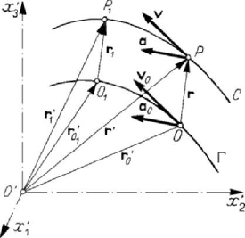
2.2.1 Motion of translation
We say that a rigid solid is subjected to a motion of translation if an arbitrary straight
bar of it remains parallel to itself at any moment of the motion. In particular, the axes
i
Ox , 1, 2, 3i = , of the movable frame of reference R must enjoy this property; as a
matter of fact, it is sufficient that the three axes do remain parallel to themselves (hence,
the moving frame of reference must have a displacement parallel to itself), in order that
any other straight line do enjoy the same property (because any straight line of the rigid
solid is rigidly connected to the frame
R ). The position vector r remains constant in
the relation (5.2.1) (it has a displacement parallel to itself), in this case; the trajectory
C
of the point
P
is obtained from the trajectory
Γ
of the point
O
by a translation of
vector
0
′′
=−
rr r (Fig.5.12). If the point
O
attains the point
1
O
on the curve
Γ
, then
the point
P
attains the point
1
P
on the curve
C
, while the vector
11 1
OP =
J
JJJG
r
is
equipollent to the vector
r .
Figure 5.12. Motion of translation of a rigid solid.
Taking into account Poisson’s formula (A.238), it results that
j
=
i0, 1, 2, 3j = , if
and only if
=ω 0 ; in this case, the distribution laws of the velocities and accelerations
are given by
Kinematics
311
O
′
′
=
vv,
O
′
′
=
aa.
(5.2.11)
Hence, at a given moment, all the points of a rigid solid in a motion of translation have
the same velocity and the same acceleration; the respective vectors may be modelled by
free vectors. If the velocity
O
′
v is given, then the equation of the trajectory becomes
0
0
() ( ) ( )d
t
t
tt ττ
′′ ′
=+
∫
rr v
(5.2.12)
If
vers const
O
′
=
J
JJJJG
v , then the motion of translation is rectilinear; otherwise, it is
curvilinear. If
const
O
′
=
v , then the motion of translation is uniform.
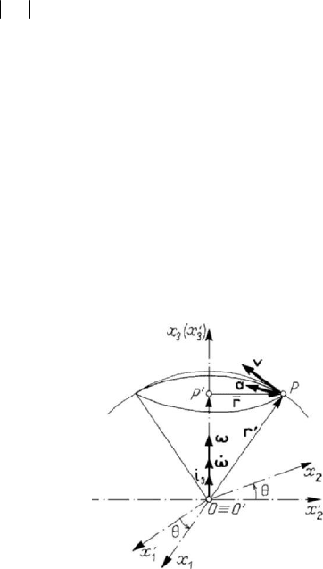
2.2.2 Motion of rotation
We say that a rigid solid is subjected to a motion of rotation if two points of it remain
fixed during the motion; the straight line which links the two points (called axis of
rotation) is fixed too, in this case. We assume (without losing from the generality of the
study) that
OO
′
≡
and we choose as axis of rotation
33
Ox Ox
′
′
≡
. The rigid solid
remains with only one degree of freedom, which is the angle
()tθθ
=
(5.2.13)
between the axes
Ox
α
′′
and Ox
α
,
1, 2α
=
(Fig.5.13). Noting that the unit vectors of
the movable frame may be expressed with the aid of the unit vectors of the fixed frame
of reference in the form
Figure 5.13. Motion of rotation of a rigid solid.
′′
=+
iii
112
cos sinθθ,
′
′
=
−+iii
212
sin cosθθ,
′
=
ii
33
the formula (A.2.36) leads to
==
12
0ωω , ==
3
() () ()tttωωθ
,
(5.2.13')
MECHANICAL SYSTEMS, CLASSICAL MODELS
312
hence, the vector
ω is a sliding vector situated along the axis of rotation
(
= i
3
() ()ttωω ), being the angular velocity vector. Thus, we have put in evidence the
mechanical significance of the vector
ω
, formally introduced in the formula (5.2.3).
The velocity of a point of the rigid solid is thus given by
PO
=
=×= ×
J
JJG
ω
ωvr r
(5.2.14)
and can be considered to be the moment of the vector
ω
with respect to the point P .
Multiplying scalarly this relation by the vector
r and by the vector
3
i
, respectively,
and noting that one obtains null mixed products, one gets
2
1d
0
2d
r
t
⋅= =
rr
,
33
d
()0
dt
⋅
=⋅=
ir ir
,
wherefrom
2
constr = and
(
)
3
,const
=
) ir . It follows that the trajectory of a point
P
is the intersection of a sphere of centre
O
and r radius and a cone, the vertex of
which is at
O
too; hence, these trajectories are circles situated in planes normal to the
axis of rotation, having the centres in points
P
′
on the very same axis. Because
OP OP P P OP
′′ ′
== + = +
J
JJJG JJJJG JJJJG
J
JJG
rr
, where P
′
is the projection of the point
P
on the
axis of rotation, one can write the relation (5.2.14) also in the form
=
×vr
ω
,
v ω
=
r
; (5.2.14')
comparing this formula with the formula (5.1.41), which corresponds to the circular
motion of a particle, we see that the velocity vector is tangent to the trajectory in the
normal plane to the axis of rotation. Noting that the vectors
r and v are polar vectors,
it results that
ω is an axial vector; besides, the above considerations justify the
denomination given to this vector. Taking into account the considerations in Chap. 3,
Subsec. 1.2.3, we may attach to the vector
ω
an antisymmetric tensor of second order,
given by the formula (3.1.62'); we write
ij
ijk k
ωω=∈ ,
1
2
i
ijk jk
ωω=∈ ,
(5.2.15)
and the relations (5.2.14), (5.2.14') become
ijjij
ijk k
vxxωω
=
∈=,
12
vxω
=
− ,
21
vxω
=
,
3
0v
=
, (5.2.14'')
so that all the points of the rigid solid have the same angular velocity. We notice that
the points on the axis of rotation are the only ones of vanishing velocity, while the
velocity vectors of the points of a straight line parallel to this axis are equipollent; as
well, the velocities are parallel and their moduli have a linear variation for the points of
a normal to the axis of rotation. Taking into account (A.2.31'), (A.2.31''), the relations
curl 2
=
v
ω
, div 0v
=
(5.2.16)
Kinematics
313
hold, the field of velocities being thus solenoidal.
Rivals formula (5.2.6''') leads to
22
ωω=×− =×−
arr rrωω
,
42
a ωω=+
r
,
(5.2.17)
corresponding to the formula (5.1.41'), which gives the distribution of accelerations in
the circular motion of particle; we have
2
ij i
ijk k
axxωω=∈ −
,
1, 2, 3i
=
,
2
121
axxωω=− −
,
2
21 2
ax xωω=−
,
3
0a
=
,
(5.2.17')
so that the accelerations are contained in a plane normal to the axis of rotation and
directed towards the interior of the circular trajectory. The determinant of the
homogeneous system which gives the points of null acceleration is
42
0ωω+≠
and
allows to affirm that only the points of the axis of rotation enjoy this property (it is one
of the cases mentioned in Subsec.2.1.1, the angular acceleration vector
=
εω being a
sliding vector too, the support of which is the same axis of rotation. As in the case of
the velocities, the accelerations are equipollent vectors for the points of a straight line
parallel to the axis of rotation; as well, for the points of a straight line normal to the axis
of rotation, the velocities are parallel, their modulus having a linear variation. If
=
0
ω ,
then the motion of rotation is uniform. If the vectors
ω
and
ω
have the same direction,
then the motion is accelerated; otherwise, it is decelerated.
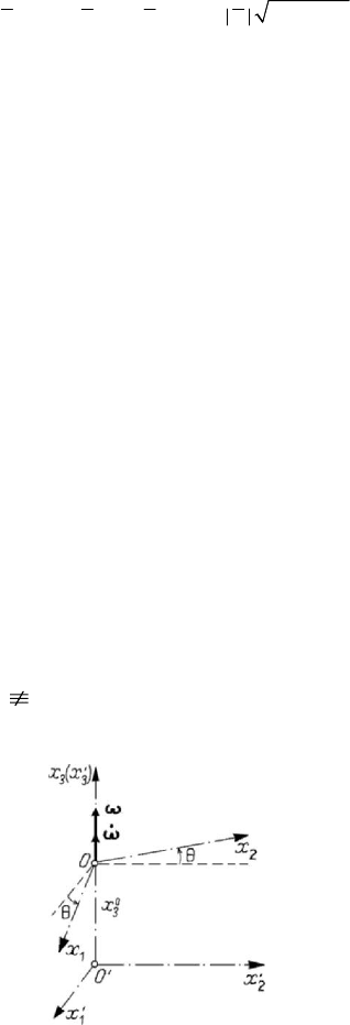
2.2.3 Helical motion. Motion of rototranslation
We say that a rigid solid has a helical motion if two of its points remain on a fixed
straight line during the motion; we may also say that a straight line rigidly linked to the
rigid solid (axis of rotation and sliding) maintains its support fixed (or slides along a
fixed support). We choose the axis of rotation and sliding as axis
3
Ox
′
′
and the point O
on this axis (in general,
OO
′
), so that the axis
3
Ox coincides with it. This motion is
defined by the scalar functions (Fig.5.14)
Figure 5.14. Helical motion of a rigid solid.
33
()
OO
xxt
′′
=
, ()tθθ
=
,
(5.2.18)
MECHANICAL SYSTEMS, CLASSICAL MODELS
314
which specifies the position of the rigid solid at a given moment (the rigid solid has two
degrees of freedom). The distribution of the velocities is given by
O
′′
=+×
vv r
ω
,
222
O
vv rω
′′
=+
,
12
vxω
′
=−
,
21
vxω
′
=
,
33
O
O
vv v
′
′′
==
,
(5.2.19)
where
() ()ttωθ=
has the significance given at the previous subsection. The formulae
(5.2.19) show that the modulus of the velocity is minimal (equal to
O
′
v ) for the points
of the axis of rotation and sliding; in fact, the velocity
()
OO
t
′
′
=
vv is a function of
time, so that one may have points of null velocity only – eventually – for some
particular cases. As in the case of a motion of rotation, the velocities of the points of a
straight line parallel to the axis of rotation and sliding are equipollent vectors. In a plane
normal to the axis of rotation and sliding we obtain a component of the velocity which
has a behaviour analogous to that in case of a motion of rotation; the component of the
velocity along the direction of the same axis behaves as in the case of a motion of
translation.
The distribution of the accelerations is given by
2
O
ω
′′
=+×−
aa r r
ω ,
()
2422
O
aa rωω
′′
=++
,
(5.2.20)
leading to the same components
1
a
′
,
2
a
′
as those given by the formula (5.2.17') and to
the component
0
3
aa
′′
= . As in the case of the velocities, the modulus of the
acceleration is minimal (equal to
0
a
′
) for the points of the axis of rotation and sliding;
but there cannot be points of null acceleration, excepting – eventually – for some
particular moments (case mentioned in Subsec. 2.1.1). We notice that
33
() () () ()ttt tωθ== =
iiεω is the angular acceleration, the same for any point of
the rigid solid. The accelerations are equipollent vectors for the points of a straight line
parallel to the axis of rotation and sliding. The component of the acceleration which is
contained in a plane normal to the axis of rotation and sliding has a behaviour
analogous to that in case of a motion of rotation; while the component of the
acceleration along the same axis has a behaviour analogous to that of a motion of
translation.
From the above considerations, it results that the helical motion can be obtained,
from the point of view of the distribution of the velocities and accelerations, by the
composition of a motion of rotation with a motion of translation along the axis of
rotation. We notice that the vectors
()
O
t
′
v and ()t
ω
have the same constant direction
(
()
O
t
′
×=v0
ω
).
The considered motion is called helical, the trajectory of a point of the rigid solid
being situated on a circular cylinder. If the first of the scalar functions (5.2.18) which
defines the motion verifies a relation of the form
3
O
xkθ
′
=
, k being a constant the
dimension of which is a length, then the trajectories are helices and we have to do with
a screw motion; the rigid solid has – in this case – only one degree of freedom. We
obtain
O
vkω
′
=
,
O
akω
′
=
, so that
Kinematics
315
22
vrkω=+,
()
24 2 2 2
ar rkωω=++
.
(5.2.21)
The pitch of the helix is
2pkπ= , so that
2
O
p
v ω
π
′
=
,
2
O
p
a ω
π
′
=
.
(5.2.22)
We notice that the helical motion is a particular case of a motion of rototranslation,
i.e., the case in which the vectors
ω
and
O
′
v have the same support. In the general
case,
O
′
×≠
v0ω , ω and
O
′
v having fixed directions, and we obtain an arbitrary
motion of rototranslation (called also motion of finite rototranslation), which is not a
helical motion; this case is basic for the study of the general motion of the rigid solid.
The relations (5.2.16) remain still valid in the case of a motion of rototranslation.
2.2.4 Motion of Frenet’s and Darboux’s trihedra
If we know the trajectory of a point of the rigid solid, then we may choose as
movable frame of reference Frenet’s trihedron. Taking into account Poisson’s formulae
(A.2.38) and Frenet’s formulae (4.1.10)-(4.1.10''), and noting that
ddd
ddd
s
tst
=
ττ
,
ddd
ddd
s
tst
=
ν
ν
,
dd
d
ddd
s
tst
=
ββ
,
we may write
d
d
v
t
ρ
=×=
τ
ω
τν
,
d
d
v
tv
ρ
ρ
=×=− −
′
ν
ω
ντ
β
,
d
d
v
t
ρ
=×=
′
β
ωβ
ν ,
(5.2.23)
which leads to interesting kinematic interpretations for the radii of curvature and
torsion. In this case, the angular velocity vector is given by
τν
β
ωωω
=
++ωτν
β
,
v
τ
ω
ρ
=
−
′
, 0
ν
ω
=
,
v
β
ω
ρ
=
(5.2.24)
and we may write
22
11
vω
ρρ
=+
′
.
(5.2.24')
In the case of a torsionless motion, hence in the case in which the trajectory of a point
of the rigid solid is a plane curve, we have
MECHANICAL SYSTEMS, CLASSICAL MODELS
316
v ρω
=
. (5.2.24'')
Analogously, choosing as a movable frame of reference Darboux’s trihedron
(assuming that we know a surface on which moves a point of the rigid solid, for
instance a cylinder in the case of a motion of rototranslation) and using the formulae
(A.2.38) and (4.1.25), as well as observations analogous to those above, we obtain
d
d
gn
vv
t ρρ
=×= +
gn
τ
ωτ
,
d
d
gg
vv
t ρρ
=×=− −
′
g
gn
ωτ,
d
d
ng
vv
t
ρρ
=×=− +
′
n
n
g
ωτ
;
(5.2.25)
we are thus led to interesting kinematic interpretations for the radii of normal curvature,
as well as of geodesic curvature and torsion. We may express the angular velocity
vector in the form
gnτ
ωωω=++
g
nωτ
,
g
v
τ
ω
ρ
=−
′
,
g
n
v
ω
ρ
=−
,
n
g
v
ω
ρ
=
,
(5.2.26)
wherefrom
222
111
gg n
vω
ρρ ρ
=++
′
.
(5.2.26')
2.3 General motion of the rigid solid
We consider, in the following, the general motion of the rigid solid as an
instantaneous helical motion, introducing the fixed and the movable axoids; according
to the form of the axoids (conical or cylindrical), we obtain the motion of a rigid solid
with a fixed point or the plane-parallel motion of the rigid solid, respectively.
2.3.1 Instantaneous helical motion. Static-kinematic analogy
In the general case of motion of a rigid solid we use the results given in Subsecs
2.1.1 and 2.1.2 concerning the distribution of velocities and accelerations. Using the
formula (5.2.3), which gives the velocity
′
v of a point P of the rigid solid with respect
to a fixed frame of reference, and the formula (5.2.14), we observe that
{
}
,{}
OO
′
=
τvωω,
{
}
,{}
PP
′
=
τvωω, with
PO O O
PO OP
′′ ′ ′
=+×=+×=+×
J
JJG JJJG
vv v v rωω ω.
(5.2.27)
We obtain thus a torsor of the angular velocities,
ω
playing the rôle of the resultant
vector (an axial, sliding vector), while
′
v is the moment resultant vector (a polar,
Kinematics
317
bounded vector). This observation stays at the basis of the static-kinematic analogy,
which allows the kinematic study of the motion of the rigid solid with the aid of the
static methods. Analysing the distribution of the velocities, we see that – at a given
moment – the general motion of a rigid solid may be identified with an instantaneous
motion of rototranslation, characterized by an instantaneous torsor of the angular
velocities.
Hence, the general motion of a rigid solid is characterized by the vectors
ω and
O
′
v
(the components of the torsor {}
O
τ
ω
of the angular velocities with respect to the pole
O , rigidly linked to the rigid solid); in general, these vectors are not collinear. There
exist points (which can belong to the rigid solid or not) for which
O
′
& v
ω
, the general
motion of the rigid solid becoming thus an instantaneous helical motion. Indeed, taking
into account the scalar of the torsor
PO
′
′
⋅
=⋅vv
ω
ω ,
(5.2.28)
which is an invariant, it follows that
PO
′
′
=
vv
<<
, where we have emphasized the
components parallel to the vector
ω
of these vectors. The formula (5.2.27) becomes
PO
⊥⊥
′
′
=
+×vv r
ω
,
(5.2.29)
where the components of the velocities normal to the vector
ω
have been introduced.
Using the method of determination of the central axis (emphasized in Chap. 2, Subsec.
2.2.5), we put the condition
P
⊥
′
=
v0, wherefrom
2
O
λ
ω
′
×
=+
v
r
ω
ω
;
(5.2.30)
we obtain thus the instantaneous axis (the locus of the searched points) with respect to
which we have an instantaneous helical motion. This axis is parallel to the vector ω ; a
vector equipollent to the latter one, the support of which is the instantaneous axis, is
called Chasles’ vector. We may write the equation (5.2.30) also in the form (a vector
product by
ω
eliminates the scalar λ )
2
O
O
ω
′
⋅
′
−× =
v
vr
ω
ω
ω ;
(5.2.30')
in components one has
()()
12332 23113
12
11
OO
vx x vx xωω ωω
ωω
′′
−+ = −+
()()
31221 112233
2
3
11
OOOO
vx x v v vωω ω ω ω
ω
ω
′′′′
=−+= ++
.
(5.2.30'')
We notice that the instantaneous axis, defined by the equations (5.2.30)-(5.2.30''), is the
locus of the points for which, at a given moment, the modulus of the velocity is
minimal. The above considerations allow us to state
MECHANICAL SYSTEMS, CLASSICAL MODELS
318
Theorem 5.2.3 (Chasles). The general motion of a rigid solid at a given moment may
be identified with an instantaneous helical motion about an instantaneous axis of
rotation and sliding.
We can say that this helical motion is tangent to the general motion of the rigid solid
at a given moment.
From the above analysis it follows that if
=
0
ω
,
O
′
=
v0, then the rigid solid is in
rest. If
=
0ω ,
O
′
≠
v0, then a motion of translation takes place; if ≠ 0ω ,
O
′
=
v0,
then the motion of the rigid solid can be identified with a motion of rotation about an
instantaneous axis of rotation passing through the fixed point
O
(in particular, a finite
rotation), hence with a rigid solid with a fixed point. If
≠
0
ω
,
O
′
≠
v0, then two cases
may occur: if the torsor’s scalar vanishes (
0
O
′
⋅
=v
ω
), then the motion of the rigid
solid is an instantaneous motion of rotation about an instantaneous axis of rotation
(which does not pass through a fixed point); if the scalar does not vanish (
0
O
′
⋅≠
vω ),
then a general motion of the rigid solid takes place.
In the general motion of the rigid solid, the distribution of accelerations is that
emphasized in Subsec. 2.1.2.
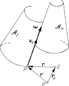
2.3.2 The fixed and the movable axoids
We notice that the instantaneous axis of rotation and sliding varies both with respect
to the fixed and the movable frames of reference, because
ω
and
O
′
v are functions of
time. The locus of the instantaneous axes of rotation and sliding with respect to the
frame
′
R is a ruled surface
f
A
, called the fixed axoid, while the locus of the same
axis with respect to the frame
R is a ruled surface
m
A
too, called the movable axoid
(Fig.5.15); these two surfaces play an important rôle in the general motion of a rigid
solid, as it was emphasized by Poncelet.
Figure 5.15. Fixed and movable axoids of a rigid solid.
Let
P be a point of the rigid solid on the instantaneous axis of rotation and sliding,
rigidly linked to this axis, for which a relation of the form (5.2.1) takes place.

Kinematics
319
Differentiating with respect to the frame
′
R and using the formula (A.2.37), we
obtain
d
d
dd
O
ttt
′
∂
=
++×
∂
r
rr
r
ω ;
(5.2.31)
d/d
P
t
′′
=vr is the velocity of the point P in the motion of the instantaneous axis of
rotation and sliding with respect to the frame
′
R , while /
P
t
=
∂∂vr is the velocity
of the same point in the motion of this axis with respect to the frame
R. Noting that
d/d
OO
t
′′
=vr and
O
λ
′
+×=vr
ω
ω , where λ is a scalar, because the translation
velocity of the point
P and the angular velocity
ω
are collinear vectors for the points
of the instantaneous axis of rotation and sliding, we get the relation
PP
λ
′
−
=vv
ω
.
(5.2.31')
If the velocities
P
v and
P
′
v would be equal, then the axoids would have a motion of
rolling without sliding; because of the vector difference
λ
ω
, occurs also a sliding of the
movable axoid on the fixed one along the direction of the vector
ω
, with the velocity
λω . Projecting the relation (5.2.31) on a direction normal to the vector ω, we obtain
PP
⊥
⊥
′
=
vv,
(5.2.32)
the components normal to the instantaneous axis of rotation and sliding of the velocities
of a point
P of this axis with respect to the fixed and movable frames of reference,
respectively, being equal. We may thus state
Theorem 5.2.4. The general motion of a rigid solid takes place so that the movable
axoid be tangent to the fixed axoid along the instantaneous axis of rotation and sliding
(the common generatrix of the two axoids), its motion being a rolling about this axis,
over the fixed axoid, together with a sliding along the same instantaneous axis.
We notice that the two axoids must be both developable or warped surfaces.
The motion of the movable axoid characterizes thus completely the general motion
of the rigid solid.
2.3.3 Motion of the rigid solid with a fixed point
In the case of a rigid solid with a fixed point both origins may coincide with this
point, without losing anything of the generality (
OO
′
≡
); we have thus
OO
′
==
vv0,
OO
′
==
aa0, the vectors
ω
and
ω
being arbitrary. The rigid solid
remains with three degrees of freedom and its position at a given moment may be
specified with the aid of Euler’s angles
,,ψθϕ, emphasized in Chap. 3, Subsec. 2.2.3.
The distribution of the velocities is given by the relation
=
×vr
ω
, (5.2.33)