Teodorescu P.P. Mechanical Systems, Classical Models Volume I: Particle Mechanics

Подождите немного. Документ загружается.

MECHANICAL SYSTEMS, CLASSICAL MODELS

340

where the angular velocity and acceleration are given by the formulae (5.3.7'), (5.3.15'),

respectively.

We mention that the formula (5.3.19) may lead to a torsor of the angular

accelerations, less useful that the torsor of the angular velocities, because of its

complicated form.

3.3 Kinematics of systems of rigid solids

After some general considerations concerning the systems of rigid solids (called also

multibody systems, where it is understood that the bodies are rigid ones), we introduce

the notion of mechanism, as an example of such systems; the results thus obtained allow

to present some applications concerning the transmission of displacements, velocities

and accelerations.

3.3.1 Systems of rigid solids

The results obtained for the relative motion of a rigid solid may be used also for

systems of rigid solids. Let be thus two rigid solids

S and

′

S , bounded by two

convex surfaces

S and S

′

, respectively, which at any moment t , have the same

tangent in an ordinary common point

′

≡

, PS

∈

, PS

′

∈

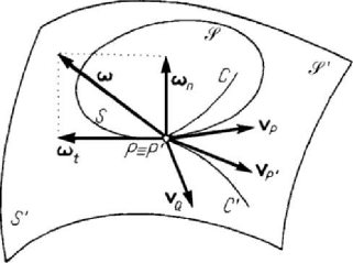
(Fig.5.29); we assume

that the solid

′

S is fixed, while the solid S is movable, remaining at any moment in

contact with the solid

′

S . Let us suppose that a movable point Q coincides with

′

≡ at any moment t ; the locus of the point Q with respect to the movable

surface

S is a curve C , its velocity

v being a relative velocity, and with respect to

the fixed surface

′

a curve C

′

, its velocity

v , being an absolute velocity. Taking

into account the relation (5.3.3), we obtain the velocity of the point

Q as a velocity of

transport with respect to the surface

′

in the form

Figure 5.29. Motion of a rigid solid over another rigid solid.

′

−vvv

. (5.3.21)

Because the velocities

′

v and

v are contained in the common tangent plane, the

velocity

v which characterizes the sliding of the surface S over the surface S

′

will

Kinematics

341

belong to the same plane. The distribution of the velocities is known if, besides the

velocity

()

tv , the angular velocity ()t

, which passes through the point P , is also

given. The motion of the rigid solid

S with respect to the rigid solid

′

S is thus

characterized by a translation of velocity

()

tv and by a rotation of angular velocity

()tω . The vector ()tω may be decomposed in two components: an angular velocity

()

tω , along the normal to the tangent plane, which characterizes a pivoting about the

respective axis, and an angular velocity

()

, contained in the tangent plane, which

characterizes a rolling about the corresponding axis. We can say that the general motion

of the rigid solid

S over the rigid solid

′

S takes place so that the surface S is rolling

and pivoting with sliding over the surface

′

. If

()

, then the motion of the

rigid solid

S over the rigid solid

′

S is an instantaneous rotation (pivoting and

rolling) about an instantaneous axis of rotation passing through the point of contact.

The fixed axoid intersects the surface

′

after the curve C

′

, while the movable axoid

intersects the surface

after the curve

; in this case,

′

vv, so that the curve

is rolling without sliding over the curve

′

during the motion. If

≠

v0 but

= 0ω

(

=ωω), then the surface S is rolling with sliding over the surface S

′

, along an

instantaneous axis of rotation and sliding; if

v0 too, then the motion is only a

rotation without sliding.

Let be the frames

R ,

R ,…,

. rigidly linked to the rigid solids

S ,

S ,…,

, respectively. Denoting by

the angular velocity in the motion of the frame

with respect to the frame

R and by (/ )

∂

∂ V the derivative with respect to time of a

vector

V in the frame

R , we may write

∂∂

=+×

∂∂

VV Vω ,

1,2,..., 1in

−

∂

+×

∂∂

VV Vω ;

summing with respect to

i and noting that the vector V is arbitrary, we obtain the

relation (equivalent to the relation (5.3.7'))

21 32 , 1 1,

...

nn n−

++ + =0ωω ω ω , (5.3.22)

which links the relative rotations of

n rigid solids. In particular, one obtains the

remarkable relations

ij ji

+=0ωω ,

ik kj

=+ωωω, ijki

≠

≠≠, , , 1, 2,...,ijk n

. (5.3.22')

Starting from

MECHANICAL SYSTEMS, CLASSICAL MODELS

342

ij ij ji ij

OO OO OO

∂∂

=+×

∂∂

JJJJGJJJJJG JJJJJG

ω ,

ij i j

−

JJJJG

rr,

we find also the relation

ij ji ij i ji j

+×+×=vv r r0ωω , ij

≠

, , 1,2,...,ij n

, (5.3.23)

complementary to the first relation (5.3.22'), where

v is the velocity of the pole

O of

the frame

R with respect to the pole

O of the frame

. Starting from the relation

(5.3.7) and using the relation (5.3.23), we get the relation

1, 1, 1, 1 1, 1

ii n ii i n

−−

+++

++ ×+×=

∑∑

vv r r0ωω

, 2n ≥ ,

(5.3.24)

corresponding to the frames

R ,

R ,…,

, the position vectors being those of a

point

P of the rigid solid with respect to the above mentioned frames. We mention that

one may write the relation (5.3.24) also in the form

1, 1, 1 1, 1 1,

ii n i ii n

PO PO

−−

+++

++ × +×=

∑∑

JJJJJG JJJJG

vv 0ωω,

2n ≥

;

(5.3.24')

the formulae (5.3.22) and (5.3.24') allow thus to use the static-kinematic analogy for the

sliding vectors

1,ii+

ω ,

1,2,..., 1in

−

, and

1,n

, the velocities

1,ii+

v ,

1,2,..., 1in=−, and

1,n

v playing the rôle of moments of those vectors.

The relation (5.3.13) may lead, on the same way, to some interesting results.

Noting that

ijijiji ij

ij j

∂∂ ∂

=+×=−

∂∂ ∂

ωωωω ω

we obtain the relation

ij ji



ω . (5.3.25)

The relation (5.3.15') allows to write

1, 1, 1,1 2, 1

ii n i ii

−−

++++

++ ×

∑∑



ωω ωω

(5.3.26)

in this case; in particular, one obtains

ik kj ik kj

+−×



ωωωωω. (5.3.25')

Using a relation of the form (2.1.50'), as for the distribution of velocities, and starting

from the relation (5.3.15), we get a relation of the form

Kinematics

343

1, 1, 1, 1, 1, 1,

111

nnn

tt CC

ii n ii n ii n

iii

−

++ +

===

++ ++ +

∑∑∑

aa aa aa

11, 11,

iii n

PO PO

+×+×+

∑

JJJJJG JJJJG



ωω

21,12,1

()

ii ii

−

++++

×=

∑

JJJJJG

0ωω ;

(5.3.27)

thus, the formulae (5.3.26), (5.3.27) lead also to the static-kinematic analogy for the

sliding vectors of the nature of angular accelerations, where the relative accelerations,

the accelerations of transport and the accelerations of Coriolis play the rôle of moments

of those vectors.

Analogous results can be obtained starting from the relation (5.3.19) too.

We consider also a mechanical system made up by three rigid solids

S ,

S and

S , which have a plane-parallel motion. The rigid solid

S has a motion of rotation

with respect to the rigid solid

S about an instantaneous axis of rotation, normal to the

plane of motion at the instantaneous centre of rotation

I , with an angular velocity

ω ; analogously, one introduce the instantaneous centres of rotation

I and

I , as

well as the corresponding angular velocities

and

. Taking into account the

second relation (5.3.22'), there results that the three parallel vectors are also coplanar, so

that one may state

Theorem 5.3.11 (theorem of the three instantaneous centres of rotation). If a

mechanical system made up by three rigid solids

S ,

S and

S has a plane-parallel

motion, then the three instantaneous centres of rotation

I ,

I and

corresponding

to their relative motions are collinear.

We notice that

ij ji

II≡ , hence the instantaneous centre of rotation of the rigid solid

S with respect to the rigid solid

coincides with the instantaneous centre of

rotation of the rigid solid

S with respect to the rigid solid

S .

3.3.2 Kinematic chains. Mechanisms

The rigid solids which constitute a system of rigid solids are called elements; one of

those elements may be considered fixed, the other elements being – in general –

movable. The link which restricts the motion of an element with respect to another one

is called kinematic couple relative to the two elements; one may say also that this is the

possibility to transmit the motion from one element to another one. Among the

kinematic couples we mention: the articulation (it allows the rotations), the coulisse or

the slideway (it allows the displacement in a given direction) and the simple support (it

does not allow displacement in a given direction). An element of a kinematic couple is

considered fixed, studying – in fact – the relative motion of the second element with

respect to the first one. The conditions of linkage (the restrictions of the relative

motion) diminish the number of degrees of freedom of the free element (which is six).

We denote by

c the number of the conditions of linkage; if 0c

, then the elements

are free one with respect to the other, while if

, then the two elements are built in

one into the other (rigid constraint). Hence

15c

≤

≤ ; if N is the number of degrees

MECHANICAL SYSTEMS, CLASSICAL MODELS

344

of freedom which remain, then we have

6cN

− . We may thus classify (after

Malyshev) the kinematic couples in five classes, after the number of the conditions of

linkage. We mention thus the plane-sphere and the plane-plane couple (of class I and

class II, respectively), the spherical and the plane couple (of class III), the annular and

the cylindrical couple (of class IV), the couple of rotation, of translation and the helical

couple (of class V); for instance, the plane-sphere couple allows two translations and

three rotations, while the cylindrical couple allows only a translation and a rotation. If

the relative motion of the two elements is a plane-parallel motion, then we have to do

with a plane couple; otherwise, the couple is a space one. In another classification, we

have: inferior kinematic couples, if the contact zone is a surface, and superior kinematic

couples, if the contact zone is a line or a point.

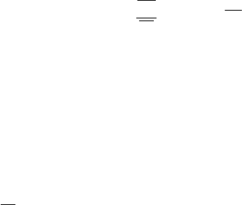
A system of rigid solids (elements) linked by kinematic couples, which allow the

motion from one element to the other, by successive transformations, is called a

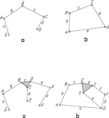
kinematic chain. If there is at least a singular element, which belongs to only one

kinematic couple, then the kinematic chain is called open (Fig.5.30,a); otherwise (if

each element of it belongs at least to two kinematic couples), the kinematic chain is

called closed (Fig.5.30,b). A kinematic chain is simple if each element of it belongs at

the most to two kinematic couples (Fig.5.30). Otherwise, the kinematic chains are

Figure 5.30. Kinematic chains: open (a) and closed (b).

complex, having at least an element involved in more than two kinematic couples; these

chains may be open or closed too (Fig.5.31,a,b). If all the couples are plane, then the

kinematic chain is plane; otherwise, it is spatial. We call basis of the kinematic

Figure 5.31. Complex kinematic chains: open (a) and closed (b).

chain an element of it which is considered fixed; the other elements are leading elements (if

they induce the motion coming from the exterior to the other elements) or followers

(if they receive the motion from the first elements). A kinematic chain for which at any

Kinematics

345

position of one or several leading elements of it corresponds a unique position for all

the other followers (with respect to the considered basis) is called desmodromous;

otherwise, the kinematic chain is called non-desmodromous. For instance, the

articulated quadrangle of vertices

,,,ABC D and sides ,,,abcd (Fig.5.32), for which

a is the basis, while the element

is leading is a desmodromous kinematic chain, the

elements

c and

being followers. In analogous conditions, an articulated pentagon,

e.g., is a non-desmodromous kinematic chain.

The number of degrees of freedom of a kinematic chain, constituted of

n elements,

linked by

n couples of class c , 1,2,...,5c

, is given by

Nn cn

=−

∑

(5.3.28)

If one of the elements of the kinematic chain is a basis, then its degree of mobility is

specified by the Somov-Malyshev formula (the structural formula of the kinematic

chains)

6( 1)

Mn cn

=−−

∑

(5.3.28')

the kinematic couples being independent. If there exist

l restrictions of motion (due,

for instance, to some anterior common linkages), then we have

(6 ) ( )

Nlncln

=− − −

∑

(5.3.29)

the degree of mobility being given by Dobrovolski’s formula

(6 )( 1) ( )

Mln cln

=− −− −

∑

(5.3.29')

In the plane case (

3l = ), we get

32Nnn n

−− and

3( 1)Mn=−−

2n− , the latter formula being due to Chebyshev.

A closed kinematic chain which has a basis and is subjected to a desmodromous

motion is called a mechanism; the number of its leading elements is – in general – equal

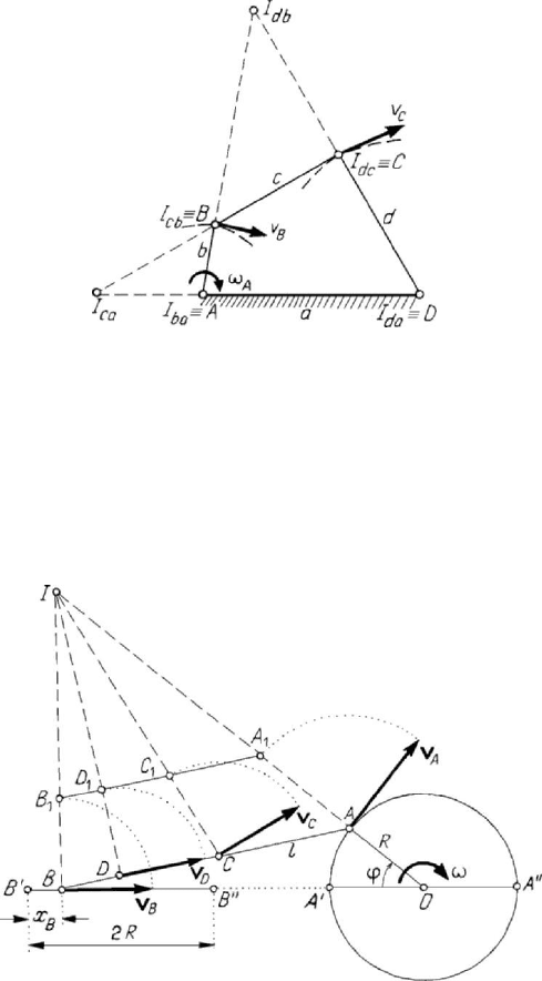
to the number of its degrees of mobility. In the case of the articulated quadrangle

( 4n = ,

0n = ,

4n = ) (Fig.5.32), Chebyshev’s formula gives 3(4 1)M =−

24 1−⋅ = . In this particular case, we distinguish six centres of rotation, i.e.: four

centres of permanent rotation (the fixed centres of rotation

≡

and

ID≡ and

the movable centres of rotation

≡

and

≡

) and two instantaneous centres

of rotation

I and

I ; corresponding to the Theorem 5.3.11, we notice that the above

mentioned centres of rotation are three abreast on the four sides of the quadrangle. In

general, a mechanism made up of

n elements has (1)/2nn

−

centres of rotation; if

MECHANICAL SYSTEMS, CLASSICAL MODELS

346

the mechanism is a polygon, then

n centres are permanent (two of them being fixed),

while

(3)/2nn

−

are instantaneous ones.

Figure 5.32. Desmodromous articulated quadrangle.

3.3.3 Applications to the transmission of displacements, velocities and

accelerations

The determination of the kinematic characteristics of a mechanism (i.e., the

positions, the velocities and the accelerations of its points) is of particular importance in

the study of it; the methods of computation used are analytical, graphical, or grapho-

analytical ones.

Figure 5.33. Crank and connecting-rod mechanism.

Let be, for instance, the crank and connecting-rod mechanism

BAO (one of the

most usual mechanisms, which transforms a rectilinear motion in a circular one)

(Fig.5.33). the leading element is the crank

AO , articulated at

and of length R ,

Kinematics

347

the position of which is specified by the angle

ϕ with respect to the position OA

′

corresponding to the dead-point (dead-position); in the latter case, the extremity

B of

the connecting-rod

BA , which glides at B and is of length l , is at the point B

′

Taking the point

′

as origin for the displacements, the position of the point B at a

given moment will be

(

)

(1 cos ) 1 1 sin

xBBR lϕλϕ

′

==− +−−

The ratio

λ being subunitary (in general, 1/3λ

), we may use binomial’s formula

for the radical, so that

(

)

22 2

(1 cos ) sin 2 sin 1 cos

222

ϕϕ

ϕϕ λ

≅− + = + .

(5.3.30)

Hence, one has the velocity

(

)

sin sin 2 sin (1 cos )

vv v

ϕϕ ϕλϕ=+ = +,

vRω

, ωϕ=  .

(5.3.31)

We must have

cos cos 2 0ϕλ ϕ+= for

maxB

v , wherefrom

()

cos 1 1 8

ϕλλ

=−++ ≅, 90ϕ

° ,

using the same approximation method as above; consequently,

()

max

11 1

vvv

λλ

⎛⎞ ⎛⎞

≅− + ≅+

⎜⎟ ⎜⎟

⎝⎠ ⎝⎠

(5.3.31')

For

1/5λ = we obtain 78 27 47ϕ

′

′′

≅

° and

max

1.02

≅

The acceleration is given by

(cos cos 2 ) sin (1 cos )

aR Rωϕλϕωϕλϕ=+++



(5.3.32)

In case of a constant regime (

constω

), it results

(cos cos2 )

aa ϕλ ϕ=+,

aRω= .

(5.3.32')

We get

max

(1 )

aaλ=+ for 0ϕ

° and

min

(1 )

aaλ

−− for 180ϕ =°; we

can also have

min

(1 )/ 8

aaλλ=− + too for cos 1/ 4ϕλ

− .

Another analytical method is the method of independent cycles, at the basis of which

stay the formulae (5.3.22) and (5.3.24'), allowing to write two vector equations of

equilibrium for each independent cycle of the considered mechanism; in the case of

MECHANICAL SYSTEMS, CLASSICAL MODELS

348

independent cycles, one may write

2n vector equations to determine the velocities

1,n

v ,

1,ii+

v and the angular velocities

1,n

1,ii+

1,2,..., 1in

−

. The formulae

(5.3.26), (5.3.27) lead to an analogous method of computation for the distribution of

accelerations. But the analytical methods are difficult to use in the case of more intricate

mechanisms.

Among the graphical or grapho-analytical methods we mention – first of all – the

method of connecting-rod curves to determine the displacements of the points of

elements of this nature.

To determine the velocities, one can use – sometimes – the method of the

instantaneous centre of rotation; for instance, in the case of the just considered crank

and connecting-rod mechanism (Fig.5.33), the centre

I can be easily obtained, so that

ωω= ,

ICωω= ,

(5.3.33)

for an arbitrary point

C of the driving rod. The velocities’ turning down method,

emphasized in Subsec. 2.3.4, allows to determine graphically the magnitude and the

direction of velocities; taking into account Fig.5.19, we may obtain the drawing of

Fig.5.33. The point

D , the foot of the normal from I to the connecting-rod AB , is the

point of minimal magnitude of the velocity, which has the direction of the connecting-

rod, and is its characteristic point. We mention that it is not necessary to obtain

previously the point

I ; that is an advantage of the latter method. But if this point is

specified and a particular scale for the velocities is chosen, so that the magnitude of the

velocity of a point be equal to the corresponding instantaneous radius (in our case

vIA= ), then the velocities of all the points will have the moduli equal to the

corresponding instantaneous radii; this is the method of the normal velocities. Euler’s

formula (5.2.3') leads to the method of the relative motion (the method of the vector

equations). As well, the formulae (5.2.4), (5.2.4') stay at the basis of the method of

velocities’ projections; thus, if we know the velocities of the points

A and B , which

correspond to two elements of a mechanism, then we may obtain the projections of the

velocity of a point

C , rigidly linked to each of the points A and B and non-collinear

with these points, on the straight lines

AC and BC , hence obtaining the velocity of

the point

C . The drawing of the velocities’ plane and the similarity theorem (for

velocities) lead to the method of velocities’ polygon for a plane-parallel motion. Using

the theorem of the three instantaneous centres of rotation (see Subsec. 3.3.1), one may

often determine the distribution of the velocities in the case of a plane mechanism (the

method of collinearity of the instantaneous centres of rotation).

To determine the accelerations of an element, we may use the graphical

representation of the accelerations of its points. As in the case of velocities, we mention

the method of relative motion (the method of vector equations), based on the formulae

(5.2.6)-(5.2.6''), the projections’ method, based on the formula (5.2.10), and the method

of accelerations’ polygon, based on the introduction of the accelerations’ plane and on

the similarity theorem (for accelerations), introduced in Subsec. 2.3.4.

We notice that a mechanism realizes a transformation of an input quantity

(displacement, velocity, acceleration) into an output quantity of the same nature; thus,

Kinematics

349

the output quantity will be equal to the input one, amplified by a coefficient, which is a

transmission ratio (or a transfer function), hence

ddλ

vvλ

, d being a

displacement and

v a velocity, where the indices o and i stay for output and input,

respectively, while

λ ,

λ are the corresponding transmission ratios. We mention that,

in the case of accelerations, we cannot speak about a transmission ratio, but only if

const

λ = , case in which

aaλ

with analogous notations; otherwise, the ratio

λ of transmission of accelerations depends not only on the position of the leading

element, but also on its velocity and acceleration.

Among the mechanisms which realize these transformations, we mention – first of

all – the mechanisms with articulated levels. One of the simplest mechanisms of this

type is the articulated quadrangle, which may be – in particular – an articulated

parallelogram. The link mechanisms may be with a translation, oscillating or rotation

link; to the first category belongs also the crank and connecting-rod mechanism, just

considered. We mention also the case in which the axle of the link does not pass

through the articulation of the crank, as well as the case of eccentric gears (for which

the ratio

/Rlλ = is very small). Another mechanism of this kind is the shaping

mechanism. The director mechanisms may be used to obtain a rectilinear or a

curvilinear trajectory; they may be reversers (exact director mechanisms) or

approximate mechanisms. The mechanisms with a Cardan joint are based on a Cardan

(universal) coupling.

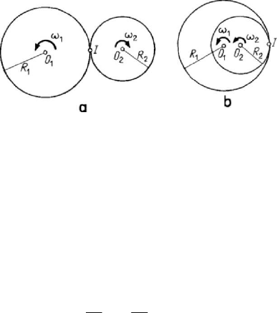
Figure 5.34. Wheel mechanisms with (exterior) (a) or interior (b) wheels.

In the case of wheel mechanisms, one must have in view the relative position of the

axes of rotation and the angular velocities; we mention that the wheels may be exterior

(Fig.5.34,a) (the rotation direction is changed) or interior (Fig.5.34,b) (the rotation

direction is maintained). The transmission may be obtained by friction wheels or by

gear wheels (trains of gears). In the case in which the axes of rotation are parallel

(Fig.5.34), having a rolling without sliding, the velocity of their point of contact (which

is an instantaneous centre of rotation too) is the same, so that the transmission ratio is

given by

==±,

(5.3.34)

where one takes the sign + or – as the direction of rotation is maintained or not; if the

motions of rotation are uniform, then we may write