Teodorescu P.P. Mechanical Systems, Classical Models Volume I: Particle Mechanics

Подождите немного. Документ загружается.

MECHANICAL SYSTEMS, CLASSICAL MODELS

240

(

)

(

)

sin cos sin cos

FG R M FG R

αϕ αϕ

⎡⎤⎡⎤

+− ≤≤++

⎢⎥⎢⎥

⎣⎦⎣⎦

;

the latter inequality specifies the minimal turning couple for which the towage is

possible, while from the first inequality one obtains the maximal traction force.

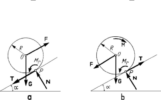
Figure 4.15. The drawn (a) and the motive (b) wheel on an inclined plane.

A hinge allows a rigid solid to effect a motion of rotation about an axis which passes

through the centre of this constraint; experimentally, one states that, applying to the

rigid solid a couple in a plane normal to the axis of rotation, the solid begins to rotate

only if this couple attains a certain limit value, because of the forces of friction which

arise. One emphasizes thus a couple of friction in the hinge,

M , which must verify the

condition of equilibrium

MfrR

′

≤

(4.2.8)

where

r is the radius of the hinge journal (we assume a cylindrical hinge), R is the

total reaction in the hinge, while

′

is a dimensionless coefficient of friction in the

hinge. The circle of radius

′

, the centre of which is at the centre of the hinge, is

called circle of friction; for equilibrium, it is necessary that the reaction

R do pierce

the circle of friction or, at the limit, be tangent to it.

Cylindrical hinges intervene in technique especially in the form of bearings. Thus,

the wheels of a machine are fixed on axle trees, which lean on bearings. The parts of

the axle trees which are in contact with bearings are called journals and are special

disposed. Because of the friction in bearings appears a moment

M , which is difficult

to be determined; indeed, the respective mechanical phenomenon is particularly

complex. Adopting the simplified hypotheses of a dry friction, one may find formulae

of the form (4.2.8), which are upper limits of the moment

M ; here, r is the radius of

the journal,

is the frictionless reaction in the axle tree, while

′

is a coefficient of

friction which depends on the type of the axle tree.

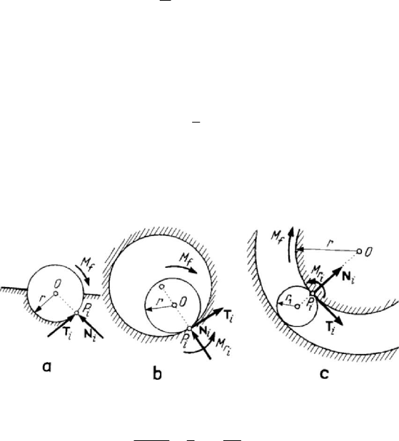
In the case of a sliding bearing we distinguish between a bearing without clearance

(Fig.4.16,a) or with clearance (Fig.4.16,b). In the first case, if we write the equation of

moment of the tangential friction forces with respect to a point of the journal axis, then

we get

Statics

241

′

∑

(4.2.9)

where

N is the normal reaction at the arbitrary point

P of contact between the journal

and the bearing, while

is the corresponding coefficient of sliding friction. In the

second case, from equilibrium conditions too, we get

′

+ ,

(4.2.9')

where

s is the coefficient of rolling friction between the journal and the bearing. In the

case of a ball contact bearing (Fig.4.16,c) one obtains a coefficient of friction

′

smaller that those obtained above; analogously, one can show that

Figure 4.16. Sliding bearing without (a) or with (b) clearance. Ball contact bearing (c).

rr R

⎛⎞

′

⎜⎟

⎝⎠

∑

(4.2.9'')

where

N is the normal reaction at a point

P of contact between the journal and the

ball,

r and

r are the radii of the journal and of the ball, respectively, while s and

represent the coefficients of rolling friction between the journal and the ball and

between the ball and the bearing, respectively.

Obviously, other cases of constraints with friction, imposed by the practice, may be

put in evidence; but all these cases reduce to a sliding, pivoting, or rolling friction or to

a combination of them.

2.1.5 Statics of systems of rigid solids

A mechanical system S constituted by a finite number of rigid solids represents a

system of rigid solids (which are considered to be

n ); we assume – in general – that the

system is subjected to constraints. Thus, the system of rigid solids may be acted upon

by given and constraint external forces (we apply the axiom of liberation from

constraints), as well as by given and constraint internal forces (between the various

component rigid solids). In general, the constraints between the rigid solids can be

simple supports, hinges, built-in supports and constraints with friction.

MECHANICAL SYSTEMS, CLASSICAL MODELS

242

l , 06ln

≤

≤ , is the number of degrees of freedom of the system,

n and

n ,

nn n≤+≤, are the number of the unknowns introduced by the external and

internal constraint forces, respectively, while

e , 06en

≤

≤ , is the number of

equations of equilibrium which may be written, then a necessary condition to determine

the statical or the instantaneous (for a mechanism) equilibrium, respectively, is of the

form

ln n e

+=. (4.2.10)

To specify the number of degrees of freedom of a mechanism is, in general, a

sufficiently difficult problem. This is a basic problem in the theory of mechanisms, but

we do not deal with it in what follows; we will suppose that the system of rigid solids is

statically determinate (the equations of static equilibrium are sufficient to determine the

constraint forces and the position of equilibrium). If the number

e of equations is not

sufficiently great, then the mechanical system is hyperstatic, and we cannot determine

all the unknowns of the problem; as for the rest, the mathematical model of rigid bodies

is – in this case – no more sufficient, and we must use a model of deformable body.

We notice that the notion of system of rigid solids is a conventional one; indeed, a

system is constituted of subsystems (parts of the system), and a subsystem

S ⊂ S

may be considered as an independent system, if only this one is of interest. Thus, the

notions of “external force” and “internal force” are relative; indeed, an internal force of

a system may be external one for a subsystem. If upon a system of rigid solids do not

act external forces, then we say that the system is isolated.

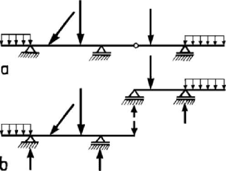
Figure 4.17. Gerber bar.

A system of rigid solids is at rest (in equilibrium) with respect to a fixed frame of

reference if any constituent rigid solid of the system is in equilibrium under the action

of all the given and constraint forces (all these forces are, for a particular rigid solid,

external forces) which act upon it. For example, let be a bar with hinges (a Gerber bar)

(Fig.4.17,a), which may be considered as being formed by two simply supported bars

(Fig.4.17,b); the Gerber bar is in equilibrium only if each of the simply supported bars

is in equilibrium. Obviously, this result is valid for any subsystem of an arbitrary

system, so that we may state

Statics

243

Theorem 4.2.2 (theorem of equilibrium of parts). If a system S of rigid solids is in

equilibrium under the action of a system of given and constraint forces, then any of its

parts (any subsystem

S ⊂ S ) is in equilibrium too under the action of the given and

constraint forces corresponding to the respective part.

Noting that the torsor of the internal given and constraint forces vanishes, we obtain

a necessary condition of equilibrium of the whole mechanical system in the form

{

}

{

}

τ+τ =FR0,

(4.2.11)

where the torsor operator is applied to all the external forces which are acting upon this

system. In this condition, which is also sufficient in the case of a non-deformable

mechanical system, the internal forces do not intervene, and that is an important

advantage for the computation. We may thus state

Theorem 4.2.3 (theorem of rigidity). Assuming that a given system of rigid solids with

constraints becomes rigid, the conditions of equilibrium of the new mechanical system

represent necessary conditions of equilibrium for the given mechanical system.

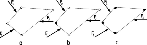
Figure 4.18. System of four bars: with four articulations (a), with one vertex

built-in (b) or with all vertices built-in (c).

It results that a deformable or non-deformable system of rigid solids, which is in rest

under the action of a given system of forces, remains further at rest if it becomes rigid

by introducing supplementary internal constraints. Thus, e.g., if a system of four

articulated bars (Fig.4.18,a) is in equilibrium under the action of the forces

123

,,,FFF

then it remains in equilibrium if the articulation of one vertex is replaced by a built-in

support (Fig.4.18,b), or if all four vertices are built-in (Fig.4.18,c).

The basic problem is – in general – a mixed problem, in which the position of

equilibrium and the constraint forces which act upon the mechanical system are

searched. If the constraints are specified by

nnm

= independent parameters

(corresponding to

m degrees of freedom which are cancelled), then the number of

independent parameters which specify the position of equilibrium will be equal to

6nm−

; in general, in the case of a statically determinate mechanical system, these

parameters may be obtained explicitly.

In the case of a system of rigid solids subjected to constraints with friction, other

problems may arise too. Let thus be the case of a system constituted of

n rigid solids,

which has only one degree of freedom and is subjected to the action of two active given

forces: the motive force

F and the resistent force

F (one may have couples of

MECHANICAL SYSTEMS, CLASSICAL MODELS

244

moments

M and

M , respectively). There exist, in general, two tendencies of

displacement, corresponding to the increasing or the decreasing of the parameter which

is fixing the position of the mechanical system. We call direct motion that one which

corresponds to the direction of displacement due to the motive force and inverse motion

that one which corresponds to the direction of displacement of the resistent force. One

determines the magnitudes of the motive force corresponding to the two tendencies of

displacement from the position of equilibrium; these two limit magnitudes depend on

the resistent force

F (or on the couple

M ), on the geometry of the static position of

equilibrium of the mechanism (distances or angles), on the fixed geometric elements

(independent of the configuration of the mechanism) and on the coefficients of friction.

The two limit magnitudes coincide if we do not take into account the phenomenon of

friction.

We say that a system of rigid solids is subjected to a phenomenon of self-fixing (or

self-braking), the position of equilibrium being maintained if the motive mechanical

element is no more acting (

F or

M ), but the resistent mechanical element (

F or

M ) still acts. We can say that the system is in equilibrium under the limit (or at the

limit) of sliding, rolling or pivoting, in the opposite tendency of a direct motion; to have

a motion in this case,

F (or

M ) must change of direction. Analogously, a system of

rigid solids is subjected to a phenomenon of self-locking if, to obtain a tendency of

direct motion, in a certain configuration of the system, the motive mechanical element

(

F or

M ) must tend to infinity. The first of these phenomena may be useful in

practice, but the second one must be avoid; thus, the study of those phenomena has a

particular importance.

Using the above exposure, we may emphasize three important methods of

computation. Thus, in the method of isolating the solids, each rigid solid of the system

is isolated by introducing the corresponding constraint forces and the conditions of

equilibrium (the torsor of the system of given and constraint forces with respect to an

arbitrary pole vanishes); there are obtained

equations of equilibrium for the

unknowns of the problem (corresponding to the position of equilibrium and to the

constraint forces). In the plane case, there remain only

equations of equilibrium.

Taking into account the principle of action and reaction, some of the unknowns may

affect two solids in linkage. The solving of the system of

equations may –

sometimes – require a very arduous computation.

In the method of equilibrium of parts, subsystems of the considered system are

isolated, introducing the corresponding external and internal given and constraint

forces, and necessary conditions of global equilibrium (the torsor of the external given

and constraint forces with respect to an arbitrary pole vanishes) are written for each

subsystem. Choosing conveniently the subsystems, one can obtain thus some constraint

forces (selecting the forces which we wish to determine) from a system of equations

with a smaller number of unknowns. In the method of rigidity (which is, in fact, a

particular case of the previous method, corresponding to the case in which the part is

the whole system), only six equations of equilibrium are written, which may be

sufficient to obtain the external constraint forces of the given mechanical system; the

application of this method as a first attempt to compute is thus justified. We notice that

the equations which are obtained by the method of equilibrium of parts or, in particular,

Statics

245

by the method of rigidity are linear combinations of the equations obtained by the

method of isolating the solids; the mechanical interpretations given above may be very

useful in computation. We notice too that the equations obtained by the method of

rigidity may be equations of verification after the method of isolating the solids has

been applied.

Figure 4.19. System of rigid solids (a) having an arborescent graph (b).

In practice, it is convenient to determine first the parameters defining the

configuration of equilibrium of the system of rigid solids; this depends on the structure

of the considered system. Conventionally, we may represent a solid of the system by a

point, while the linkage between two solids is represented by a segment of straight line,

which joins the corresponding points. A graph is thus obtained – a schema

corresponding to the structure of the system; hence, the method of graphs may be used

too.

To the system of rigid solids in Fig.4.19,a there corresponds the graph in Fig.4.19,b,

while to the system in Fig.4.20,a does correspond the graph in Fig.4.20,b; the fixed

element has been denoted by

0 . A cycle of a graph is a succession of its lines, which

forms a closed polygon. A graph which has not one cycle is called arborescent. Thus,

the graphs are of two classes: arborescent graphs (as that in Fig.4.19,b) and graphs with

cycles (as that in Fig.4.20,b, which has three cycles). In the first case, one may write the

equations which have as unknowns only independent parameters, specifying

the

Figure 4.20. System of rigid solids (a) having a graph with cycles (b).

configuration of equilibrium (in the considered case, four parameters). In the second

case, the problem can be reduced to the previous one if one transforms the given system

in a system of rigid solids with arborescent graphs, by removing some internal

connections, each of them interrupting a cycle; because there exist several possibilities,

MECHANICAL SYSTEMS, CLASSICAL MODELS

246

it is – obviously – recommendable to remove the linkages which introduce the smallest

number of scalar unknowns (for instance, between a simple support and a hinge, it is

preferable to eliminate the simple support).

2.1.6 Applications. Simple devices

In what follows, we deal – shortly – with applications of statics of rigid solids to

some well known mechanical devices, called – usually – simple devices; these ones are

used in their simplest form or in the construction of various machines or equipments.

They are rigid solids or systems of rigid solids and are subjected to two categories of

forces: motive forces, which try to put the system in motion, and resistent forces, which

are opposed to the motion. The systems of forces which act upon these devices must be

in equilibrium. In general, a simple device allows to overcome a resistent force of

greater intensity by means of a motive force of smaller intensity. Sometimes, if the aim

of the mechanical device is to change the direction of the motive force or a better

equilibration from statical point of view, then it is possible to have the same intensity

for the resistent force as for the motive one (or the intensity of the latter one may be

smaller). We deal only with simple devices with a single degree of freedom,

characterized by only one parameter of geometric nature, which specifies the position

of equilibrium. One must find the relation between the modulus of the motive force and

the modulus of the resistent force for equilibrium. In general, the own weight of these

devices is neglected, because it is small with respect to the magnitude of the considered

forces.

Although they are numerous, the simple devices can be divided in two great classes:

simple devices of the class of the inclined plane (the inclined plane, the wedge, the

screw) and simple devices of the class of the lever (the lever, the systems of articulated

levers, the apparatuses of weight, the hoists and the pulleys).

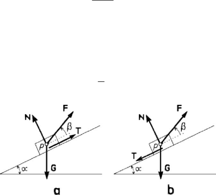
Figure 4.21. Inclined plane without friction.

The inclined plane is a simple device which allows to move up or down the solid

bodies, through the agency of a force materialized, for instance, by a cable. Let be such

a body, modelled by a particle

P of weight G which leans frictionless on an inclined

plane of angle

α (Fig. 4.21); one must determine the force F which must be applied at

the point

P , so that this one be at rest. Writing the equations of equilibrium along the

inclined plane and the normal to it, we get

cos sinFGβα= , sin cosFNGβα

= , 0N ≥ ,

Statics

247

where

is the angle made by the force F with the inclined plane, while N is the

normal reaction. The second equation determines the constraint force, while the first

one specifies the force

F ; we notice that the solution is not unique (indeed, we have

obtained only a relation between the modulus of the force

F and the direction,

characterized by the angle

β ). Because 0/2απ

≤

≤ , there results 0cos 1β≤≤

and

/2 /2πβπ−≤≤ , as well as the condition sinFG α≥ . We may also write

cos( )sec 0NG αβ β=+≥, wherefrom /2 /2πβπα

−

≤≤ −. In particular, for

0β = we obtain sinFG α= , cosNG α

, for /2βπ α

− we have 0N = ,

FG= , while for βα=− there results tanFG α

, secNG α

. In the limit case

0α =

(horizontal plane) we get /2βπ

− ,

NGF

, the modulus

being

arbitrary, or

/2βπ= ,

NGF

−

≤

; in the limit case /2απ

we obtain

secFG β= , tanNGβ=− , /2 0πβ

−

<≤. Between the motive force of modulus

FF= and the resistent force of modulus

the relation

sin

cos

(4.2.12)

takes place; if

0β = , we notice that

, and the motive force necessary to move

up a body of weight

G is smaller than the resistent force. For 0β

≠

, this relation of

order takes further place only if

αβ

(4.2.12')

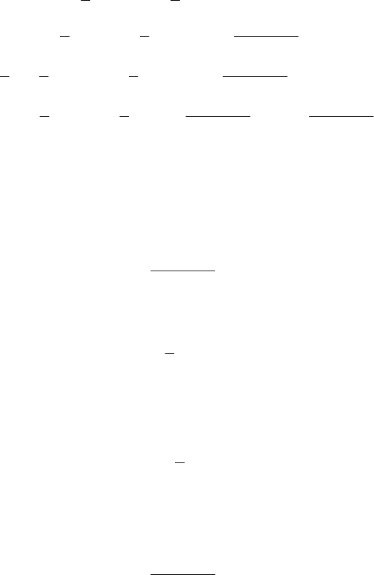
Figure 4.22. Inclined plane with friction, which hinders the particle to “move down” (a)

or to “move up” (b).

If the material point

P stays with friction on the inclined plane, the coefficient of

friction being

tan

ϕ= (Fig.4.22), we distinguish two cases, as the force of sliding

friction has a direction or another one, contrary to the tendency of sliding of the

considered body. The equations of equilibrium will be (along the inclined plane and the

normal to it)

cos sinFTGβα±= , sin cosFNGβα

= , 0 TfN

≤

≤ ,

MECHANICAL SYSTEMS, CLASSICAL MODELS

248

N being the normal reaction (the condition 0N > is included above). The first two

equations determine the constraint forces; by replacing in the third relation, one obtains

two inequalities, which put into evidence a relation between the modulus of the force

and its direction, characterized by the angle

β . If the force T hinders the particle to

“move down” along the inclined plane (Fig.4.22,a), then we obtain the condition

0 sin cos ( cos sin )GF fGFαβ αβ≤−≤ − or sin cosGFαβ≥ , as well as

sin( ) cos( )GFαϕ βϕ−≤ +; if the force T hinders the particle to “move up” along

the inclined plane (Fig.4.22,b), then we obtain the condition

0cos sinFGβα

≤

−

(cos sin)

GFαβ≤− or

cos sinFGβα≥

, as well as sin( )G αϕ+

cos( )F βϕ≥−. We consider now the particular case 0 αϕ

< . If the particle tends

to slide down along the inclined plane, then we are in the first case. Noting that

sin( ) 0αϕ−<, the second condition is fulfilled for cos( ) 0βϕ+≥ or

/2 /2πϕβπϕ−−≤≤ −; analogously, the first condition is fulfilled for

cos 0β ≤

hence for

/2πβ π−≤ ≤− or /2πβπ

≤

≤ . It follows that for /2πϕ−−

/2βπ≤≤− , F arbitrary, the equilibrium takes place. If /2 /2πβπϕ

−

<≤ −,

then the condition

sin secFG αβ≤

must hold too. For /2πβ π ϕ

−

≤<− − and

/2πβπ≤≤ we have cos( ) 0βϕ

< , and

cos 0β

≤

, hence the condition

sin( )FG αϕ≤−⋅sec( )βϕ

is sufficient. For /2 /2πϕβπ

−

<< we have

cos 0β >

, so that we associate also the condition

sin secFG αβ

≤

. Noting that

sin( )sec( )αϕ βϕ−+≶ sin secαβ, hence sin( )cos sin cos( )αϕ β α βϕ

−

+≷ ,

as we have

cos( ) 0αβ+ ≶ , there result two subcases (we remember that αϕ< ): if

/2 /2πϕβπα−<≤ − then we have sin secFG αβ

≤

, while if /2πα−

/2βπ≤< , then the condition sin( )sec( )FG αϕ βϕ

≤

−+ is imposed. In

conclusion, the equilibrium takes place for

/2πβ π ϕ

−

≤<− − or /2πα−

βπ≤≤, sin( )sec( )FG αϕ βϕ≤− + for /2 /2πϕβπ

−

−≤≤− , F arbitrary,

and for

/2 /2πβπα−<≤ −, sin secFG αβ

≤

. If the particle tends to slide up

along the inclined plane, then we are in the second case. Noting that we cannot have

cos 0β ≤ and that the second condition is verified if cos( ) 0βϕ

−

≤ , we have

equilibrium for

/2 /2πβπϕ−<≤−+, sin secFG αβ≥ . As well, for /2πϕ−+

< β < /2π , sin sec sin( )sec( )GFGαβ αϕ βϕ

≤

≤+ − we have equilibrium too;

because

sin sec sin( )sec( )αβ αϕ βϕ≤+ − only if cos( ) 0αβ

≥ , it follows that

this condition holds only for

/2 /2πϕβπα

−

+<≤ −. We have thus obtained all

the possibilities of equilibrium for

0 αϕ

< , immaterial of the tendency of sliding of

the particle. Effecting an analogous study for all the possible values of the angle

α , the

following conditions of equilibrium are obtained (immaterial of the tendency of sliding)

0 αϕ≤≤:

πβ ϕ

−≤ ≤−− or

αβπ

−

≤≤,

sin( )

cos( )

αϕ

βϕ

−

≤

Statics

249

ππ

ϕβ ϕ−− ≤ ≤−+

, F arbitrary,

ππ

ϕβ α−+ ≤ ≤ −

sin( )

cos( )

αϕ

βϕ

≤

−

;

ϕα≤≤

ππ

ϕβ ϕ−− ≤ ≤−+

sin( )

cos( )

αϕ

βϕ

−

≥

ππ

ϕβ α−+ ≤ ≤ −

sin( ) sin( )

cos( ) cos( )

GFG

αϕ αϕ

βϕ βϕ

−+

≤≤

+−

If the material point is in equilibrium for

≤

(hence if it is acted upon only by the

force

G ), then one obtains the phenomenon of self-fixation. If the equilibrium takes

place for an arbitrary

(no matter how great), then the phenomenon of self-locking is

obtained.

If the inclined plane is used to move up a body of weight

G , then the relation

−

sin( )

cos( )

αϕ

βϕ

(4.2.13)

takes place. We notice that

−+ <2

αβ ϕ ,

≤

βϕ

(4.2.13')

or if the relation (4.2.12') holds for

≥βϕ

. If

0β , then the force which moves up

the body along the inclined plane has a modulus less than the force necessary to move it

along the vertical if

αϕ .

(4.2.13'')

If the inclined plane is used to move down the heavy bodies, then the tendency of

sliding is the descending one. The formula (4.2.12) remains, further, valid; in the case

of a sliding friction, the relation

−

sin( )

cos( )

αϕ

βϕ

(4.2.14)

takes place. We notice that for

≤

αϕ,

≤

+<0/2βϕ π , we have ≤ 0

F , while

the body is self-fixed on the plane; the forces of friction are sufficient to ensure this

equilibrium.

The wedge is a dismountable simple device (a device of fixed joining), having the

form of a triangular or trapezoidal prism, which is introduced between two pieces,

acting upon them by pressure and friction forces. In the case of a symmetric wedge

(with double inclination), of vertex angle

2α (Fig.4.23), we may write