Teodorescu P.P. Mechanical Systems, Classical Models Volume I: Particle Mechanics

Подождите немного. Документ загружается.

MECHANICAL SYSTEMS, CLASSICAL MODELS

220

Otherwise, if – at a point

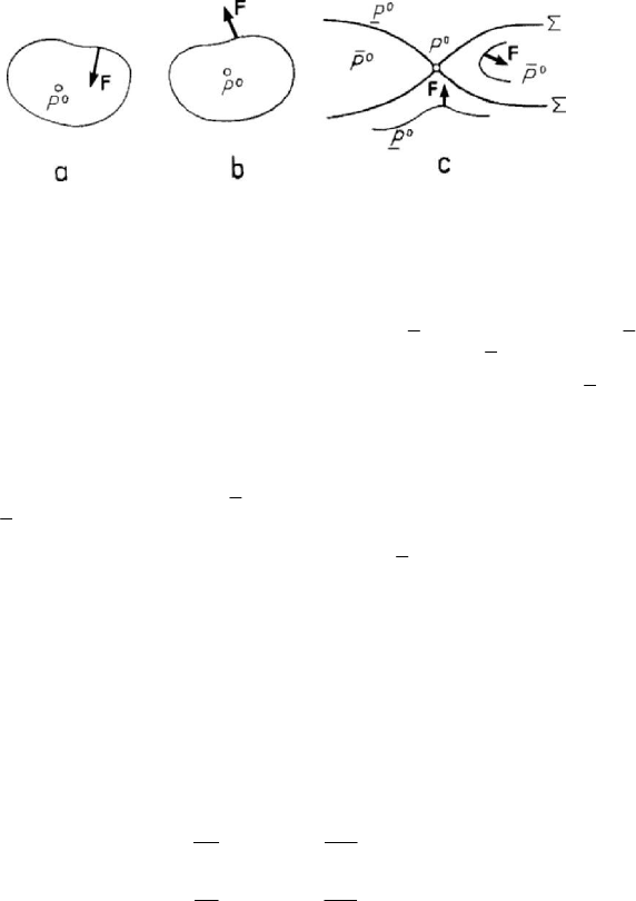
P – U reaches an isolated minimum

U , then the

equipotential surface

UU ε=+, 0ε > sufficiently small, surrounds this point,

while the force

F is normal to the mentioned surface, in the direction of the growing

U , hence towards the exterior (Fig.4.7,b); this force has the tendency to move away the

particle

P form the point

P , so that it represents a position of labile equilibrium.

Figure 4.7. Stable (a) and labile (b) positions of equilibrium.

Conical point of a level surface (c).

Let us suppose that the three equations (4.1.46) or (4.1.46') are verified at the point

, but the potential U has neither an isolated maximum, nor an isolated minimum. In

the neighbourhood of this point there exist two regions

P and

P , so that in

P the

function

takes values greater that

(the value of

P ), while in

P it takes

values smaller than

; these regions are separated by a level surface

for which

UU= and which, obviously, passes through

, where it has a conical point

(Fig.4.7,c). The force

F has the tendency to carry the particle P at the point

P , in

the region

P , while in the region

P the respective force has the tendency to move

away the particle from this position; because an arbitrary perturbation of the position of

equilibrium

may lead the particle P in the region

, it follows that this one is an

instable position of equilibrium (labile or critic equilibrium).

We notice that Torricelli’s theorem is a particular case of the Lagrange-Dirichlet

theorem.

Let be the case of a particle

P constrained to stay on a fixed smooth surface S

(Fig.4.6,a), given by the equations (4.1.29). The given force

F must be normal to the

surface at the respective point, hence to each of the co-ordinate curves

constv = and

constu = ; the conditions of equilibrium are thus of the form (

Q and

Q are called

generalized forces)

(,) (,) 0

Quv Fuv

∂

≡

⋅= =

∂∂

(,) (,) 0

Quv Fuv

∂

≡

⋅= =

∂∂

(4.1.47)

obtaining thus the values of the parameters

u and v corresponding to the searched

positions. An interesting case is that in which

ddQu Qv

is a total differential of a

function

(,)Uuv; this function is thus given by

Statics

221

(,) (,)d (,)

Uuv F uv x uv=

∫

(4.1.47')

The positions of equilibrium correspond to the points for which the function

U of two

independent variables has an extremum, hence for which

∂

, 0

∂

(4.1.47'')

In particular, if the force

derives from a potential (

,ii

, 1, 2, 3i

), then the

latter one can be obtained in the form

123 123

(, , ) (, , )d

Uxxx Fxxx x=

∫

;

(4.1.47''')

the transformation relations (4.1.29) lead to

((,)) (,)Uuv Uuv=r , the conditions of

equilibrium being of the form (4.1.47''). In general, the equipotential surface

passing

through a position of equilibrium

is tangent at the very same point to the given

surface

S , because the given force F must be normal both to this surface and to the

equipotential surface. To justify – in this case – the Lagrange-Dirichlet theorem, we

may study the form of the curves

UU ε

± , 0ε > sufficiently small, on the surface

S ,

U corresponding to the position of equilibrium.

Let us consider a particle

P constrained to stay on a fixed smooth curve C

(Fig.4.6,b), given by the parametric equations (4.1.33). The condition of equilibrium

(4.1.33''') (the given force is normal to the curve at the point corresponding to the

position of equilibrium) is of the form (

Q is called generalized force)

() () () 0

Qq F qx q

′

≡⋅ = =

(4.1.48)

obtaining thus the parameter

q which corresponds to the searched positions. Taking

into account the function

() ()d () ()d

Uq F q x q Qq q==

∫∫

(4.1.48')

the positions of equilibrium correspond to the values of

q for which the derivative

vanishes

d()

(4.1.48'')

hence, for the points of extremum of this function. If the force

is conservative, then

the potential

()U r is given by (4.1.47'''), while the transformation relations (4.1.33)

lead to

(()) ()Uq Uq=r

, the condition of equilibrium being of the form (4.1.48''). The

MECHANICAL SYSTEMS, CLASSICAL MODELS

222

study of the tendency of displacement of the particle on the curve in the neighbourhood

of the position of equilibrium may justify the Lagrange-Dirichlet theorem.

1.1.8 Particle subjected to constraints with friction

As we have seen, in general, the constraint force which acts upon a particle can be

decomposed in the form (4.1.6); in the case of an ideal constraint, the component

which hinders the particle to leave the constraint is sufficient. If the constraint is with

friction, then the component

≠

T0 hinders the particle to move along this constraint.

In what follows, we use the Coulombian model introduced in Chap. 3, Subsec. 2.2.11

for the constraint force, supposing that the constraints are scleronomic and holonomic.

We notice that this force is tangent to the rough surface or curve on which the particle

is constrained to stay; its direction is opposite to the sliding tendency, while its modulus

verifies the relation (3.2.40), the particle remaining in equilibrium.

In the case of constraints with friction, a supplementary unknown (the tangential

component

T ), for the determination of which we dispose of the inequality (3.2.40), is

thus introduced; in general, the corresponding problems are indeterminate (there are

regions on the surface or on the curve in which the equilibrium is possible). The limit

positions at which a particle remains in equilibrium may be determined in the case of a

rough curve, the inequality (3.2.40) becoming an equality; but in the case of a rough

surface, the limit positions of equilibrium are curves on this surface (in fact, the force

T has two unknown components in this case).

If the particle

P is subjected to constraints with friction, then the equation of

equilibrium is written in the form

+=FNT0; (4.1.49)

we associate to it the equation of the rough surface

S (for a particle constrained to stay

on this surface) and the inequality (3.2.40). We dispose thus of five scalar equations for

the unknowns

and

x , 1, 2, 3i

, which specify the constraint forces and the

position of equilibrium

. Taking into account (3.2.40), the relation (4.1.49) leads to

222 222

() 2TFNfN=+ = +⋅+ ≤FN FN ; projecting on the external normal n to

the surface, one obtains

= , as well as

⋅

=FN . There results

(

)

222

1NfF+≥

; the region of equilibrium on the surface S is thus specified by the

data of the problem in the form

(

)

222

FfF+≥

(4.1.50)

Noting that

222

cos

FF μ= , where μ is the angle made by the force F (or the total

constraint force

) with the normal to the surface at the position of equilibrium

P ,

and introducing the angle of friction given by (3.2.41), we obtain the geometric

condition

μϕ≤

; hence, the support of the force

(or of the constraint force

)

must be in the interior or on the frontier of the cone of friction of vertex angle

2ϕ

Statics

223

(Fig.3.32,a). If the constraint is unilateral, of the form (4.1.42), then the cone of friction

has only one sheet.

If the particle

P is constrained to stay on a rough curve C , then we must associate

the equations of the curve to the equation of equilibrium (4.1.49) and to the inequality

(3.2.40); we dispose thus of six scalar relations for the unknowns

N (equivalent to two

unknowns, the components of

N in the normal plane to the curve), T and

x ,

1, 2, 3i = , which give the constraint forces and the position of equilibrium

P . Taking

into account (3.2.40), from (4.1.49) we get

2222

() 2NFT

+=++⋅FT FT

/Tf≥ ; projecting on the tangent to the curve, we obtain 0

= , as well as

FT⋅=FT . The region of equilibrium on the curve C is thus specified by the data of

the problem in the form

(

)

2222

FffF+≤

(4.1.51)

Because

222

cos

FF μ= , where μ is the angle made by the force F (or by the

total constraint force

R ) with the tangent to the curve at the position of equilibrium

P , we find the condition

22 2

cos sin cos ( /2 )μϕ πϕ≤= −, hence the geometric

condition

/2μπ ϕ≥−, where ϕ is the angle of friction given by (3.2.41); hence, the

support of the given force

F (or of the constraint force R ) must be in the exterior or

on the frontier of the cone of friction of vertex angle

2πϕ

−

(Fig.3.32,b). In the case

of unilateral constraints, only one sheet of the mentioned zone corresponds to the

positions of equilibrium.

A synthesis of the above results is given by

Theorem 4.1.5. A particle constrained to stay on a fixed rough surface or curve

(constraints with friction) is in equilibrium if and only if the resultant of the given

forces which act upon it is contained in the interior of the cone of friction of vertex

angle

2ϕ or in the exterior of the cone of friction of vertex angle 2πϕ

−

, respectively,

or on the frontier of the cone (the case of limit equilibrium). In the plane case, the cone

of friction becomes an angle of friction.

Let be a particle

P of weight G subjected to stay on a circle of radius l ,

222

xxl+=, in a vertical plane

(Fig.4.3,b). Noting that

11 22

lx x

+ni i

and

G=−Gi

, we get

FGxl=⋅=−Gn ; we may use the formula (4.1.50), which

leads to

(

)

(

)

222 2 2

/1Gxl f G+≥. Hence, the positions of equilibrium are on the

arcs of circle

′′′

and

′′′

, specified by the relations

−≤ ≤−

≤

(4.1.52)

respectively; because

tan

ϕ=

, we may write

coslx l ϕ≤≤−

coslxlϕ

≤

(4.1.52')

MECHANICAL SYSTEMS, CLASSICAL MODELS

224

too. The two arcs on which takes place the equilibrium are contained in an angle of

vertex

O and which is equal to 2ϕ .

1.2 Statics of discrete systems of particles

Let us consider, in what follows, free or constraint discrete mechanical systems,

hence the case of a finite number of particles; We introduce the principle of virtual

work in the case of ideal constraints. The general results thus obtained may be used in

the case of continuous mechanical systems too.

1.2.1 Free discrete mechanical systems

Let S be a free discrete mechanical system, hence a finite system of n free particles

{

}

, 1,2,...,

Pi n≡=S . We suppose that a particle

P of position vector

r is acted

upon by a given external force

F (the resultant of all given external forces acting upon

this particle) and by the given internal forces

F , ji

≠

, , 1,2,...,ij n

; we notice

that the internal forces verify the axiomatic relation (1.1.81). The forces acting upon

this mechanical system are modelled by bound vectors, hence we say that the system of

particles is at rest with respect to a given frame of reference (the system of given forces

is in equilibrium or the free discrete mechanical system is in equilibrium) if the system

of bound vectors is equivalent to zero (using the principles of mechanics, as in the case

of a single particle), hence if

iij

∑

FF0, ji

≠

, 1,2,...,in

(4.1.53)

A finite system of free particles is in equilibrium if any of its particles is in equilibrium;

hence, any subsystem of the considered system will have this property (any particle

which forms this subsystem is in equilibrium). We may thus state

Theorem 4.1.6 (theorem of equilibrium of parts). If a free discrete mechanical system

S is in equilibrium under the action of given external and internal forces, then any of

its parts (any subsystem

S ⊂ S ) will be in equilibrium too under the action of the

given forces corresponding to the respective part.

Computing the torsor of the given forces and noting that the torsor of the internal

forces is equal to zero (as it was shown in Chap. 2, Subsec. 2.2.8,

{

}

τ=F0), it

follows that

{

}

=F0;

(4.1.54)

hence, a necessary condition of equilibrium is obtained by equating to zero the torsor of

the given external forces with respect to an arbitrary pole. In Chap. 2, Subsec. 2.2.2 it

was shown that, in the case of a non-deformable mechanical system, the forces are

modelled with the aid of sliding vectors; taking into account the conditions in which a

system of forces modelled by sliding vectors is equivalent to zero, it follows that, in the

Statics

225

case of a non-deformable discrete mechanical system, the condition (4.1.54) is a

sufficient condition of equilibrium too. This condition may be written in the form

i =

∑

F0,

i =

∑

rF 0.

(4.1.54')

The condition (4.1.54) has a great advantage, i.e. it does not contain the internal forces.

We may state

Theorem 4.1.7 (theorem of rigidity). Supposing that a free discrete mechanical system

S becomes rigid, the conditions of equilibrium of this new mechanical system

represent necessary conditions of equilibrium for the initially given mechanical system.

The first basic problem is that in which the forces acting upon the free discrete

mechanical system

S are given, and one must determine its position of equilibrium. In

the second basic problem, the positions of equilibrium of the particles which form the

free discrete mechanical system

S are given, and one asks to determine the forces

which act upon this system. In general, one may enunciate a mixed basic problem with

respect to the above mentioned questions. The conditions of equilibrium (4.1.53) are

equivalent to

3n scalar relations; in the case in which the considered mechanical

system is plane (from the point of view of the positions of the particles, the forces

which are acting being coplanar too), the number of these relations is reduced to

2n ,

while if the mechanical system is linear (all the particles as well as the forces are on the

same support), we may write only

n scalar relations.

1.2.2 Constraint discrete mechanical systems

Let us consider a discrete mechanical system S, hence a finite system of n particles

{

}

, 1,2,...,

Pi n≡=S subjected to m scleronomic and holonomic or non-

holonomic constraints. As in the previous case, we admit that a particle

P of position

vector

r is acted upon by the external force

F and by the internal forces

F , ij≠ ,

, 1,2,...,ij n= ; using the axiom of liberation from constraints, we introduce the

external constraint force

R (the resultant of all the external constraint forces which act

upon this particle) and the internal constraint forces

R , ij

≠

, , 1,2,...,ij n

, which

verify the axiomatic relation (1.1.81) too. All the forces which act upon the mechanical

system are modelled by bound vectors; we may say (as in the case studied in the

previous subsection) that the system of particles is at rest with respect to a given frame

of reference (in equilibrium) if

()

ii ijij

++ + =

∑

FR F R 0, ji

≠

, 1,2,...,in

(4.1.55)

Because each particle must be in equilibrium, we may state

Theorem 4.1.6' (theorem of equilibrium of parts). If a constraint discrete mechanical

system

S is in equilibrium under the action of given and constraint forces, then any of

MECHANICAL SYSTEMS, CLASSICAL MODELS

226

its parts (any subsystem

S ⊂ S ) will be in equilibrium too, under the action of the

given and constraint forces corresponding to the respective part.

Noting that the torsor of the internal given and constraint forces vanishes we obtain a

necessary condition of equilibrium in the form

{

}

{

}

τ+τ =FR0

(4.1.56)

or in the form

()

∑

FR 0,

()

iii

∑

rFR 0.

(4.1.56')

In these conditions, which are also sufficient for a non-deformable discrete mechanical

system, the internal forces do not intervene; this is an important advantage for

computation. Hence, we state

Theorem 4.1.7' (theorem of rigidity). Supposing that a constraint discrete mechanical

system

S becomes rigid, the conditions of equilibrium of the new mechanical system

represent necessary conditions of equilibrium for the initially given mechanical system.

The basic problem which arises is, in general, a mixed problem, in which the

constraint forces acting upon the given discrete mechanical system must also be

determinate. If the constraints are expressed by

m distinct scalar relations, then the

number of independent parameters which specify the position of equilibrium is equal to

3nm− ; these parameters may be obtained in an explicit form in the case of

holonomic constraints, which are thus eliminated from the computation. The system of

3n scalar relations (4.1.55) allows to determine the position of equilibrium of the

mechanical system as well as the constraint forces; but this system of equations is not

always compatible and determinate.

A discrete mechanical system of

n particles for which the equations (4.1.55) lead to

a finite and determinate solution (we have

30nm

−

≥ ) is called a statically

determinate (isostatic) system; in the case of equality, the mechanical system is at rest,

whatever given forces are acting upon it. If the system of equations is indeterminate

(the number of the unknowns of the problem is greater that the number of equations,

30nm−<), then the mechanical system is statically indeterminate (hyperstatic).

1.2.3 Principle of virtual work

Let S be a discrete mechanical system subjected to ideal constraints (for which the

virtual work of the constraint forces (3.2.36) vanishes). Starting from the necessary and

sufficient conditions of equilibrium (4.1.55), written in the form (

F and

R are the

resultants of all given and constraint forces, respectively, immaterial if they are external

or internal)

+=FR 0, 1,2,...,in

, (4.1.57)

Statics

227

performing a scalar product by the virtual displacements

r , summing for all the

particles of the system

S and taking into account the relation of definition of the ideal

constraints (3.2.36), we obtain the relation

δ= ⋅δ=

∑

Fr ,

(4.1.58)

which represents a necessary condition of equilibrium.

Supposing that the condition (4.1.58) is fulfilled and that

p constraints of the form

(3.2.21'') and

m constraints of the form (3.2.15) take place, one can use the method of

Lagrange’s multipliers; we may thus write

11 1

ii i

ll kki

il k

fλμ

== =

⎛⎞

∇+ ⋅δ=

⎜⎟

⎝⎠

∑∑ ∑

Frα ,

where

λ , 1,2,...,lp= ,

μ , 1,2,...,km

, are scalars to be determined (the

Lagrange’s multipliers) and where we notice that in a finite double sum one can invert

the order of summation. By a reasoning analogous to that given in Chap. 3, Subsec.

2.2.9, we obtain

ll kki

fλμ

+∇+ =

∑∑

F0α , 1,2,...,in

(4.1.59)

We find again the relations (3.2.37), which give the constraint forces; hence, the

relations (4.1.59) are equivalent to the relations (4.1.57). We may state (the relation

(4.1.58) is now a sufficient condition too)

Theorem 4.1.8 (theorem of virtual work). The necessary and sufficient condition of

equilibrium of a discrete mechanical system subjected to ideal constraints and acted

upon by a system of given forces is obtained by equating to zero the virtual work of

these forces for any system of virtual displacements.

Taking into account the equivalence between the relation (4.1.58), which represents

the theorem of virtual work, and the relations (4.1.57), which represent the form taken

by Newton’s principle (3.2.35') in the static case (equating to zero the accelerations

a ), it follows that the theorem of virtual work may be considered as being a principle

(the principle of virtual work or the principle of virtual displacements), because,

starting from it, one can solve the basic problems of statics.

In contradistinction to the necessary condition (4.1.56) or to the necessary conditions

(4.1.56'), where the internal forces do not appear, but the constraint forces do intervene,

in the necessary and sufficient condition (4.1.58) are involved all the given forces

(external and internal), but the constraint forces are absent; it is an advantage for the

computation, because one can specify the position of equilibrium even if the constraint

forces are not determined.

The equations (4.1.59) are called Lagrange’s equations of equilibrium of the first

kind.

MECHANICAL SYSTEMS, CLASSICAL MODELS

228

Introducing the virtual displacements (3.2.1'), we may write the condition (4.1.58) in

the form

∗

⋅

∑

Fv ,

(4.1.58')

so that the above considered principle may be called the principle of virtual velocities

too.

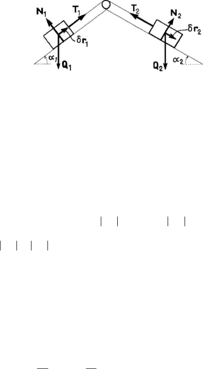
Figure 4.8. Equilibrium of two heavy bodies on inclined plains.

Let be, for instance, two solids of weights

Q and

Q , respectively, staying on two

planes inclined by the angles

α and

α , respectively, with respect to a horizontal line,

and linked by an inextensible thread, which passes over a small pulley (Fig.4.8).

Between the two bodies (which may be modelled as two particles) and the inclined

planes arise the external constraint forces

N and

N , respectively, while in the thread

appear the tensions

T and

T , respectively (internal constraint forces for the

considered mechanical system); we admit that do not appear frictions (the considered

constraints are ideal). The principle of virtual work is written in the form

11 22 11 1 22 2

sin sin 0QQαα⋅δ + ⋅δ = − δ + δ =QrQr r r ;

noting that

δ=δrr, there results the necessary and sufficient condition of

equilibrium

1122

sin sinQQαα

, (4.1.60)

which is independent of the constraint forces.

A particle

P constrained to stay on a fixed smooth surface S is specified by the

position vector

(,)uv=rr , where u and v are co-ordinates on the surface; the

principle of virtual work

(,) (,) 0uvQuvuQuvv

∂∂

⋅δ = ⋅ δ + ⋅ δ = δ + δ =

∂∂

FrF F

yields conditions of equilibrium of the form (4.1.47) for the generalized forces

Q and

Q . If the particle P is constrained to stay on a fixed smooth curve C , being specified

Statics

229

by the position vector

()q=rr , where q is a parameter, then we may write the

principle of virtual work in the form

() 0qQqq

∂

⋅

δ= ⋅ δ= δ=

∂

FrF

;

we find thus again the condition of equilibrium (4.1.48) for the generalized force.

In the case of unilateral ideal constraints of the form (3.2.16

) or of the form

(3.2.16), the virtual work of the constraint forces verifies the inequality (3.2.36'). The

principle of virtual work will be expressed in the form

=⋅δ≤

∑

(4.1.61)

for any system of virtual displacements, representing the necessary and sufficient

condition of equilibrium of a discrete mechanical system subjected to unilateral ideal

constraints; in this case too, one may make considerations analogous to those made

above.

2. Statics of solids

Among the continuous mechanical systems, we consider – in what follows – only the

solids, that is rigid solids and deformable ones. Concerning the latter ones, we deal only

with perfect flexible, torsionable and inextensible threads, as well as with bars and

systems of bars; the general study of deformable solids needs more complex

mathematical models.

2.1 Statics of rigid solids

We start with the general problem of equilibrium of free and constraint rigid solids;

the results thus obtained are then applied to various particular cases (the rigid solid with

a fixed point or axis, the rigid solid subjected to constraints with friction etc.). The

systems of rigid solids are taken into consideration too.

2.1.1 Statics of the free rigid solid

Let be a free rigid solid, hence a non-deformable continuous mechanical system

subjected to a system of given forces

{

}

, 1,2,...,

F ; these forces are external

ones. The internal forces are due to the constraints (the cohesion forces between the

particles which constitute the rigid solid) and do not intervene in computation;

moreover, the work effected by these forces vanishes.

A free rigid system may have any position in space that depends only on the system

of forces acting upon it. As we have seen in Chap. 2, Subsec. 2.2.2, the forces are

modelled by means of sliding vectors in the case of a non-deformable mechanical