Morris & Fan. Reservoir Sedimentation Handbook

Подождите немного. Документ загружается.

SEDIMENT YIELD FROM WATERSHEDS 7.21

withdrawn during both rising and falling stages of each significant event to calibrate the

turbidity data. All automatic sampling can be performed by portable battery-operated

sampling equipment with a data logger and onboard computer to program the data

collection sequences. Sampling programs established as part of a general water-quality

monitoring network are inadequate for estimating sediment load.

7.3.3 Uncertainty in Sediment Yield

Continuous long-term sediment concentration data are usually not available, and

considerable judgment is often required to convert the available data into estimates of

sediment yield. The magnitude of error that is possible in estimating sediment loads by

different practitioners can be illustrated by the lively discussion between Griffiths (1979)

and Adams (1980) concerning sediment yields from rivers draining the Southern Alps on

South Island, New Zealand. Both investigators used essentially the same dataset to

construct rating curves, but Adam's study resulted in average yields 70 percent higher

than Griffiths'. However, on the Cleddau River there was a 48-fold difference in the

sediment yield estimates. Adams points out that, because load estimates from point

concentration samples may be in error by +100 percent or -50 percent, the importance of

the 70 percent difference in yield is uncertain. That both investigators consider their

results to be "in general agreement" speaks to the high degree of variability that can occur

in fluvial sediment studies.

Galay (1987) reported that the rate of reservoir sedimentation in the Himalayas and in

India has often been underestimated for the following reasons. Sediment sampling and

analysis programs are generally inadequate to determine long-term sediment loads.

Suspended sediment measurements are often unavailable for high discharges, and there

are no measurements during catastrophic events. Bed load is not measured, and cannot be

measured accurately in large mountain rivers that may be transporting cobbles or even

boulders. Older data may reflect watershed conditions prior to extensive deforestation.

Field data may have poor quality control or may sometimes be falsified, especially at

remote and poorly supervised stations. These same limitations may apply to data from

other parts of the world as well.

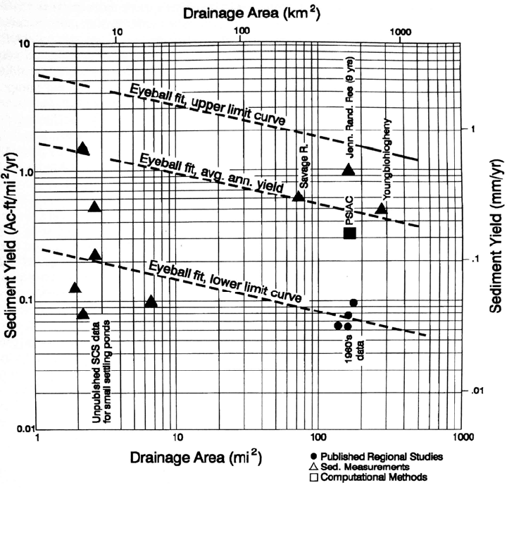
The episodic nature of sediment discharge can cause yield estimates to be severely

underestimated, especially in mountainous areas. An example of this is the case of

Jennings Randolph Reservoir on the North Branch of the Potomac River in the

Appalachian highlands in Maryland and West Virginia, described by Burns and

MacArthur (1996). The sediment yield from the 673 km

mountainous watershed was

originally estimated at 25,000 m

/yr (20 acre•ft/yr), but 2 years after impounding began

in 1982, significant sediment deposition was noticed, and in 1986 the flood of record

deposited a sediment volume equal to 30 years of sediment inflow according to the

original design computations. A resurvey after only 4 years of operation revealed that the

reservoir had already accumulated 43 percent of the projected 100-year sediment load of

2.5 Mm

The original sedimentation estimates had been based on several regional sediment

yield studies plus stream sediment samples collected during 1961-62 for river discharges

less than 140 m

/s, a recurrence interval of about 1 year. In Fig. 7.15 the measured rate of

SEDIMENT YIELD FROM WATERSHEDS 7.22

FIGURE 7.15 Various sediment yield estimates associated with Randolph Jennings Reservoi

(Burns and MacArthur, 1996).

sedi

mentation at the site is compared to various regional estimates of sediment yield,

sediment surveys at other nearby reservoirs, and an estimate prepared by the PSIAC

methodology (see Sec. 7.6.3). The scatter in the data underscores the practical problem of

attempting to assign a sediment yield to a site without reliable fluvial monitoring data.

The study concluded that the original sedimentation estimate was based on valid data,

was computed by accepted methods, and was generally in concurrence with a number of

other studies prepared in the area. However, in this mountainous watershed sediment

yield tends to be dominated by infrequent large events, and the traditional and accepted

methods for computing sediment yield can greatly underestimate sediment yield from a

basin dominated by extreme episodic events.

7.3.4 Quantifying Interannual Variability in Sediment Load

The year-to-year variation in sediment load is greater than the variation in streamflow.

Information on this variability can be used to determine the uncertainty in the estimate of

mean annual load as a function of sampling duration. Assuming that errors are not

introduced in the sampling or computational procedures, the uncertainty in estimating the

SEDIMENT YIELD FROM WATERSHEDS 7.23

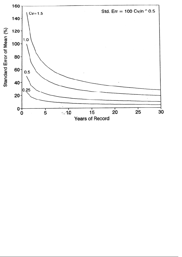
FIGURE 7.16 Timewise variation in uncertainty in estimating the mean sediment discharge.

mean

annual sediment load attributable to natural interannual variability can be

quantified as the standard error of the mean:

SE = 100 C

0.5

(7.1)

where SE = standard error of the mean suspended sediment discharge, %; C

coefficient of variation computed as the standard deviation divided by the mean; and n =

number of years of record. The timewise solution of this equation for several

representative values of C

is illustrated in Fig. 7.16, showing that the decrease in the

standard error of the mean annual load is initially rapid, but after about 10 years the error

declines rather slowly. For a stream with C

= 0.70, after 5 years of measurement the

standard error of the mean annual sediment load would be ± 31 percent, after 10 years it

would be 22 percent, and after 30 years it would be 13 percent. A 20 percent error in the

estimate of the mean due to natural variability is tolerable in most engineering studies and

is very small compared to the other types of errors inherent in sediment monitoring

programs. The use of a 5- to 10-year monitoring program has been recommended as

adequate by a number of authorities (Strand and Pemberton, 1987; Day, 1988;

Rooseboom, 1992; Summer et al., 1992). A much longer monitoring period is required to

detect trends.

7.4 SEDIMENT RATING CURVES

The relationship between sediment discharge and concentration, usually plotted as a

function of water discharge on log-log paper, is called a sediment rating curve.

Techniques for developing concentration or load versus discharge relationships have been

SEDIMENT YIELD FROM WATERSHEDS 7.24

described by Glysson (1987), who argued in favor of the term sediment transport curve,

since the term rating suggests a degree of causality that does not really exist. Rating

curves are developed on the premise that a stable relationship between concentration and

discharge can be developed which, although exhibiting scatter, will allow the mean

sediment yield to be determined on the basis of the discharge history.

Two types of relationships are commonly used, concentration versus discharge and

load versus discharge. Because sediment yield is the product of both concentration and

discharge, in the latter curve the discharge term appears on both axis, and produces an

apparent fit which is better than the original dataset. Plots of field data represent

essentially instantaneous concentration-discharge data pairs, but curves may also be

plotted showing average sediment concentration or load as a function of discharge

averaged over daily, monthly, or other time periods.

7.4.1 Fitting Sediment Rating Curves

A concentration versus discharge rating curve in some streams may be characterized by a

single log-log relationship. When there is a poor relationship between concentration and

discharge, a better relationship might be obtained by constructing multiple curves to

model different components of the total load. For instance, separate curves may be

prepared for the coarse and fine size classes, for summer and winter conditions, for rising

and falling stages or for different discharge ranges. A problem inherent in the rating

curve technique is the high degree of scatter, which may be reduced but not eliminated.

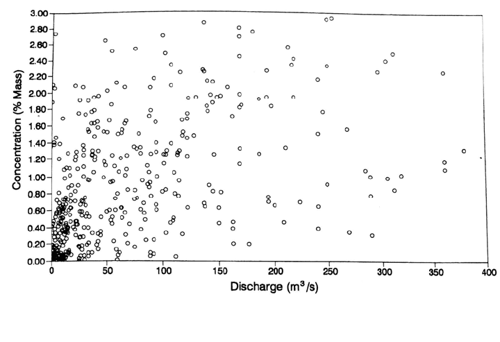
Concentration does not necessarily increase as a function of discharge (Fig. 7.17). Scatter

FIGURE 7.17 Variation in discharge and suspended concentration in the Mississippi River a

Chester, Illinois, during the 1993 flood, showing a large drop in suspended solids concentration

with increasing discharge (Holmes and Oberg, 1996).

some stations may be so great as to preclude the development of a reliable rating

relationship (Fig. 7.18). A high degree of scatter occurs when sediment delivery to the

stream is controlled by processes in the watershed that do not correlate well with the

stream discharge.

There is no standard method for rating curve construction, and in some cases visual

fitting methods can give better results than mathematical curve fitting. Construction of a

rating curve should always begin by analyzing a simple plot of the data to look for

relationships (e.g., seasonal effects) that may not be apparent from a mathematical curve-

fitting procedure. The case study on Cachí reservoir (Chap. 19) provides a good example

of how multiple methods are used to produce rating curves. A good curve fit does not

SEDIMENT YIELD FROM WATERSHEDS 7.25

FIGURE 7.18 Suspended sediment concentration versus discharge, Caledon River a

Jammersdrift, South Africa (Rooseboom, 1992).

ply an accurate representation of the hydrologic process unless the data: (1) cover the

entire range of discharges, (2) include both rising and falling stages of hydrographs from

storms during all seasons, (3) are not biased by unusual hydrologic conditions, (4)

include points at high discharge for more than a single event.

7.4.2 Visual Curve Fitting

Visual curve fitting has long been used for the construction of rating curves and can have

several advantages over mathematically fitted curves. High-discharge events which

transport most sediment are often poorly represented in sediment datasets, and data from

the highest-discharge classes may be absent altogether. Extrapolation into the highest-

discharge classes is probably better achieved by visual fitting from an experienced

practitioner as opposed to extrapolation of a regression relationship. Complex relation-

ships may also be visually broken into subsets to yield a better relationship than a single

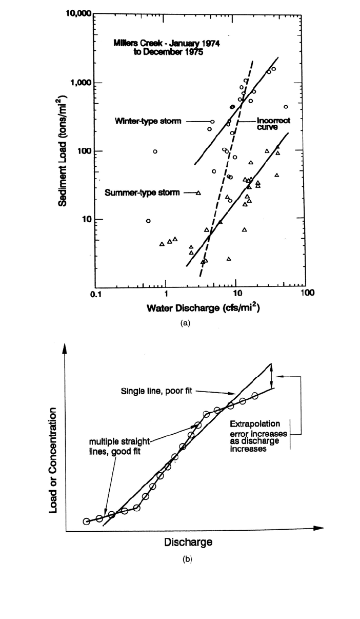
fitted curve. Two such strategies are illustrated in Fig. 7.19. Other possible strategies

include subdivision of the dataset into rising and falling stages, or preparation of separate

rating curves for coarse and fine sediment. The rating curve may also shift significantly

following an extraordinary flood which scours out the sediment stored in stream chan-

nels.

7.4.3 Mathematical Curve Fitting

A rating curve may be constructed by log-transforming all data and using a linear least

square regression to mathematically determine the line of best fit. The log-log relation-

ship between concentration (or load) and discharge is of the form C

= aQ

, and the log-

transformed form will plot as a straight line on log-log paper:

log





blog(Q) (7.2)

SEDIMENT YIELD FROM WATERSHEDS 7.26

FIGURE 7.19 Disaggregation of discharge-concentation data pairs into subsets to better define

the relationship. (a) Disaggregation of dataset by season or type of storm. (b) Use of multiple line

segments to better fit an unusual distribution. This method may be particularly useful whe

group-averaged data are used (adapted from Glysson, 1987).

SEDIMENT YIELD FROM WATERSHEDS 7.27

However, a regression equation will minimize the sum of the squared deviations from the

log-transformed data, which is not the same as minimizing the sum of the squared

deviations from the original dataset, and this introduces a bias that underestimates the

concentration (or load) at any discharge. To illustrate this effect, consider the values of 10

and 90, which have a mean value of 50. If these values are log-transformed, their logs

averaged, and the antilog of the average back-transformed, the resulting mean is 30.

Because the geometric mean computed by using the log transforms will necessarily be

lower than the arithmetic mean, the result is a negative bias, the magnitude of which

increases with the degree of scatter about the regression. Ferguson (1986) reports that this

bias may result in underestimation by as much as 50 percent. Ferguson and others have

suggested bias correction factors, but their appropriateness is uncertain (Glysson, 1987;

Walling and Webb, 1988).

Alternatives to the lognormal transformation are now widely available with

microcomputer technology. McCuen (1993) provides a description of several alternative

procedures plus software diskettes containing programs and sample datasets, which allow

the power model to be fit so that the error term is minimized on the basis of the original

unlogged dataset. Another method for testing the goodness of fit of different models

against the original dataset of instantaneous concentration-discharge was used by Jansson

(1992a) at Cachí reservoir. In this case the total load for the original dataset was

computed by assigning an arbitrary duration interval to each sample point. The total load

was then recomputed by each model (regression, visual fit, etc.) using all the discharge

values contained in the original dataset, to see how accurately each model reflected the

total load for the sampled period.

A particular weakness of a mathematically fitted curve is the potentially poor fit at the

high extreme, which will be represented by few datapoints. Large errors can occur when

mathematical curves (e.g., a log-quadratic) are extrapolated to discharge values greater

than those covered in the original dataset, producing unreasonable values. All rating

curves should be plotted and examined for reasonableness over the entire range of

discharge values to which they will be applied.

The infrequent large-discharge events which account for most sediment load will

constitute only a few points in the entire sediment dataset. As a result, the shape of a

regression equation fit using the original dataset will be biased by the numerous data-

points at low discharge values, which account for a small percentage of the sediment

load. This problem can be overcome by dividing the data into discharge classes,

computing the mean sediment concentration within each discharge class, then running the

regression model using the means. This technique equally weighs the error minimization

scheme over the entire range of the dataset.

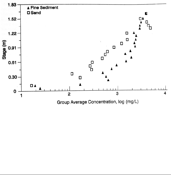
7.4.4 Rating Curve Example

As an example, the 8-year C-Q record at 21 km

Goodwin Creek, Mississippi, was

divided into 0.076-m (0.25-ft) stage intervals using discharge and suspended sediment

data pairs from a gaging flume equipped with a pumped sampler. The dataset was divided

between the fine and sand fractions, and the mean suspended sediment concentration for

each fraction was determined for each stage interval to produce the plot in Fig. 7.20,

which illustrates the clearly separate relationships for sand and fines. Although the

resulting relationship appears to imply a high degree of correlation between discharge

and concentration, the original dataset displays considerable scatter. The standard

deviation of concentration within a stage interval is about as large as the average

concentration itself. Application of the averaged data may accurately determine the long-

term load, but estimates for individual storms would incorporate large errors. In this

SEDIMENT YIELD FROM WATERSHEDS 7.28

FIGURE 7.20 Suspended sediment rating relationship for Goodwin Creek, Mississippi, from

interval-average datapoints. Note the different relationships for the fine and coarse fractions.

(Willis et al., 1989.)

waters

hed it was possible to obtain more accurate curves for the analysis of seasonal

transport rates by constructing four seasonal rating curves for 3-month periods, for both

sand and fines, for a total of eight rating curves. There was a greater seasonal effect on

the transport of fines than of sand (Willis et al., 1989).

7.5 COMPUTING SEDIMENT LOAD

7.5.1 Time-Series Sediment Rating Curve Technique

If a reliable rating relationship is available, the suspended-sediment load may be

computed by using a rating curve and a time series of discharge data. The product of

discharge and discharge-weighted concentration equals load during the computational

interval, and daily sediment load Q

in either metric tons or short tons may be computed

Metric units:

= 0.0864CQ

water

(7.3)

U.S. customary units:

= 0.0027CQ

water

(7.4)

where Q

water

is in either m

/s or ft

/s and suspended sediment concentration C is in mg/L.

Rating curves developed from short periods of sediment gaging are often applied to long-

term (e.g., 30-year) streamgage records to determine long-term sediment yield. This time

series analysis can be used to determine the seasonality of sediment discharge as well as

SEDIMENT YIELD FROM WATERSHEDS 7.29

the long-term yield. For a seasonal analysis, seasonal shifts in the rating relationship

should be incorporated if they are significant.

In sediment yield computations, the time base of rating relationships should always

match that of the discharge data for computing sediment yield. Thus, a rating relationship

between daily load and mean daily discharge would be used to compute load from a daily

discharge series. A rating curve based on instantaneous C-Q data pairs should be applied

to mean daily discharge only when concentration is changing so slowly that an

instantaneous value is representative of the 24-h interval. Application of a rating curve

constructed from instantaneous C-Q data to a mean daily discharge series can

underestimate sediment yields by 50 percent on smaller streams because the average

daily flows do not reflect the peak discharges (Walling, 1977).

7.5.2 Load-Interval Flow-Duration Technique

Either annual or seasonal flow-duration data may be used to determine the long-term and

seasonal sediment yield. In this case, a load-interval method is used to determine the

sediment load within each discharge interval, instead of constructing a rating curve. The

load interval procedure consists of two steps:

1. The discharge axis of the rating curve is partitioned into intervals and the average

load for each class is calculated as the mean of the individual loads associated with

the datapoints in the class. Approximately 20 classes may be used.

2. The total load for the period of record is computed as the sum of the mean load for each

discharge interval multiplied by the discharge frequency for the same interval.

This method was found to produce a significant improvement in the accuracy of the

period-of-record load estimate compared to the rating curve technique, because the mean

load associated with a particular discharge class reflects only samples in that class and is

not influenced by trends in adjacent classes as in a rating curve (Walling and Webb,

1981).

7.5.3 Interpolation Procedures

Interpolation uses time series sample points for suspended sediment and discharge to

compute total load, assuming the measured values represent the mean values in each time

interval. When short time intervals are used (e.g., 10 to 15 min. on small streams) this is

the most accurate method available for determining load, since it continuously tracks the

actual variation in both concentration and discharge. For continuous monitoring, turbidity

has been used to gage concentration, and pumped samples may be used to continuously

recalibrate turbidity against concentration. Procedures for turbidity monitoring are

discussed in Chap. 8. Although the interpolation procedures can be used only over a

period in which discharge and suspended sediment are monitored simultaneously, they

can be used to construct rating relationships (e.g., daily load versus daily discharge) that

can subsequently be applied to a longer-term discharge dataset.

7.5.4 Estimating Bed Load

Bed load is usually not measured, but is estimated as a fraction of the suspended sediment

load. Strand and Pemberton (1987) present a procedure outlined in Table 7.4 for

estimating bed load.

SEDIMENT YIELD FROM WATERSHEDS 7.30

TABLE 7.4 Bed Load Correction to Suspended Load Data

Suspended

sediment

concentration, mg/L

Streambed

material

Texture of

suspended material

Bedload in terms of

suspended load, %

<1000 Sand 20-50% sand 25-150

1000-7500 Sand 20-50% sand 10-35

>7500 not sand* <25% 5-15

Any concentration Clay and silt No sand <2

*Includes compacted clay, gravel, cobble, and boulder streambeds.

Source: Strand and Pemberton (1987).

7.6 ESTIMATING SEDIMENT YIELD

Estimates of sediment yield may seek to determine: the long-term yield, the timewise

variability in sediment load for the design and modeling of a sediment routing procedure,

or the spatial variability in sources of sediment to better focus yield-reduction efforts. A

recent summary of techniques for estimating sediment yield was prepared by MacArthur

et al. (1995).

This section introduces methods for estimating sediment yield that can be used at

ungaged sites as well as gaged sites. However, even sophisticated computational methods

can be based on heavily biased data, such as a nonrepresentative sediment rating curve,

and computational sophistication is not synonymous with accuracy. It is always good to

use multiple methods as a check. As an example of how multiple methods can be used to

estimate sediment yield, MacArthur et al. (1990) used the results from a prior study, data

from six nearby reservoirs, a published sediment yield map, and four different

computational procedures (flow-duration, PSIAC, Dendy and Bolton drainage area

relationship, and computed bed load for the erodible channel) to estimate sediment yield

at Caliente Creek in California, an ephemeral stream incised into a semiarid alluvial fan

and characterized by highly episodic sediment discharge.

Future conditions can differ from the present. New reservoir construction upstream,

sediment release from upstream reservoirs, land use and geomorphic change, and

catastrophic events all complicate the issue of long-term yield predictions, and the

fallibility of long-term projections must always be kept in mind. Sediment yields usually

seem to be underestimated. For example, Tejwani (1984) reviewed sedimentation studies

of 21 Indian reservoirs and found that the specific sediment yield was lower than

projected in one reservoir, but ranged from 40 to 2166 percent higher than the design

value at the remaining 20 sites. Much of the problem was attributed to degradation of the

watershed following project design studies. In contrast, the inflow of sediment into Lake

Mead on the Colorado River has been far less than originally predicted due to a long-term

reduction in sediment yield plus the construction of upstream storage reservoirs.

7.6.1 Regional Rate of Storage Loss

The results of reservoir surveys within a region may be used to estimate the overall rate

of storage loss per unit of tributary area. This is a simple procedure in which measured

specific sediment rates at other reservoirs in the regions (expressed in 10

/km

/yr, or

mm/yr) are plotted against drainage area to develop a regional relationship, as illustrated

Morris &amp; Fan. Reservoir Sedimentation Handbook

Подождите немного. Документ загружается.

Morris & Fan. Reservoir Sedimentation Handbook