Morris & Fan. Reservoir Sedimentation Handbook
Подождите немного. Документ загружается.

SEDIMENT YIELD FROM WATERSHEDS 7.31
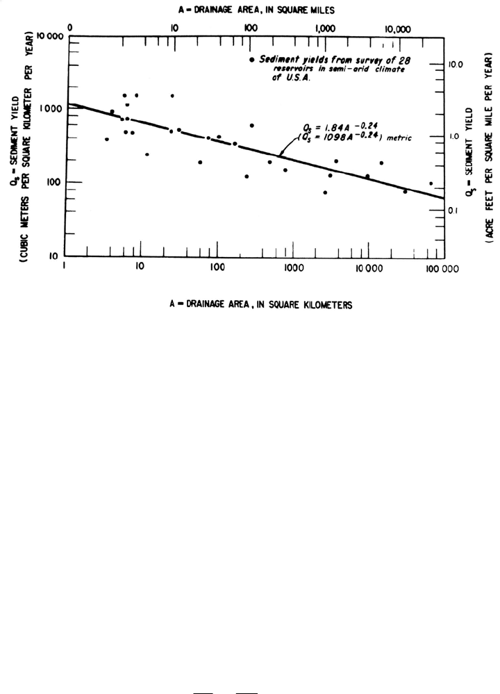
FIGURE 7.21 Average annual sediment yield versus drainage area size for semiarid areas in the
estern United States (Strand and Pemberton, 1987). w
in
Fig. 7.21. The resulting relation will provide a guideline for estimating the anticipated
sedimentation rate at the subject site. In preparing a graph of this type it is essential that
the reservoirs all occupy watersheds having geologic and land use conditions similar to
the site under investigation. Not all reservoirs in a general geographic area will be similar
and as a result this approach will produce a very credible relationship in some regions but
it may not work at all in others.
7.6.2 Regional Regression Relationship
If data on sediment yield and watershed characteristics are available from many sites, it
may be possible to develop a regression relationship which describes the sediment yield
within the region as a function of independent variables such as watershed area, slope,
land use, and rainfall erosivity.
Dendy and Bolton (1976) related specific sediment yield to drainage area using
resurvey data from about 800 reservoirs throughout the United States (excluding Florida),
for drainage areas from 2.5 to 78,000 km
2
and runoff depths up to 330 mm/yr. Sediment
yield was related to drainage area by the following relationship:
S
S
R
A
A
R
0.16
(7.5)
At 505 sites, data were also available on mean annual runoff. It was found that the
specific sediment yield peaked at about 508 mm (2 in) of annual runoff, resulting in two
equations for predicting sediment yield based on both runoff depth and drainage area. For
sediment depths less than 508 mm/yr:

SEDIMENT YIELD FROM WATERSHEDS 7.32
RRR
A
A
Q
Q
C
S
S
log 26.043.1
46.0
1
(7.6)
For runoff depths over 508 mm/yr:
R
QQ
R
A
A
eC
S
S
R
log 26.043.1
)/11.0(
2
(7.7)
In the above three equations the following terms are used with values given in metric
(and U.S. customary) units:
A = watershed area, km
2
(mil)
A
R
= reference watershed area value, 2.59 (1.0)
C
l
= coefficient, 0.375 (1.07)
C
2
= coefficient, 0.417 (1.19)
Q = runoff depth, mm/yr (in/yr)
Q
R
= reference runoff depth value, 508 mm/yr (2 in/yr)
S = specific sediment yield, t/km
2
/yr (ton/mi
2
/yr)
S
R
= reference specific sediment yield value, 576 t/km
2
/yr (1645 ton/mi
2
/yr)
Observed versus computed sediment yields for the 505 sites were plotted from Eqs. (7.6)
and (7.7), producing a correlation coefficient of r
2
= 0.75.
These equations express only the general relationship between drainage area, runoff,
and sediment yield and should be used only for preliminary planning purposes or as a
rough check. Because these equations reflect average conditions across the United States,
actual yields will tend to be higher (or much higher) than predicted in erosive areas and
lower than predicted in areas of undisturbed watershed. Local site-specific conditions can
influence sediment yield much more than drainage area or runoff.
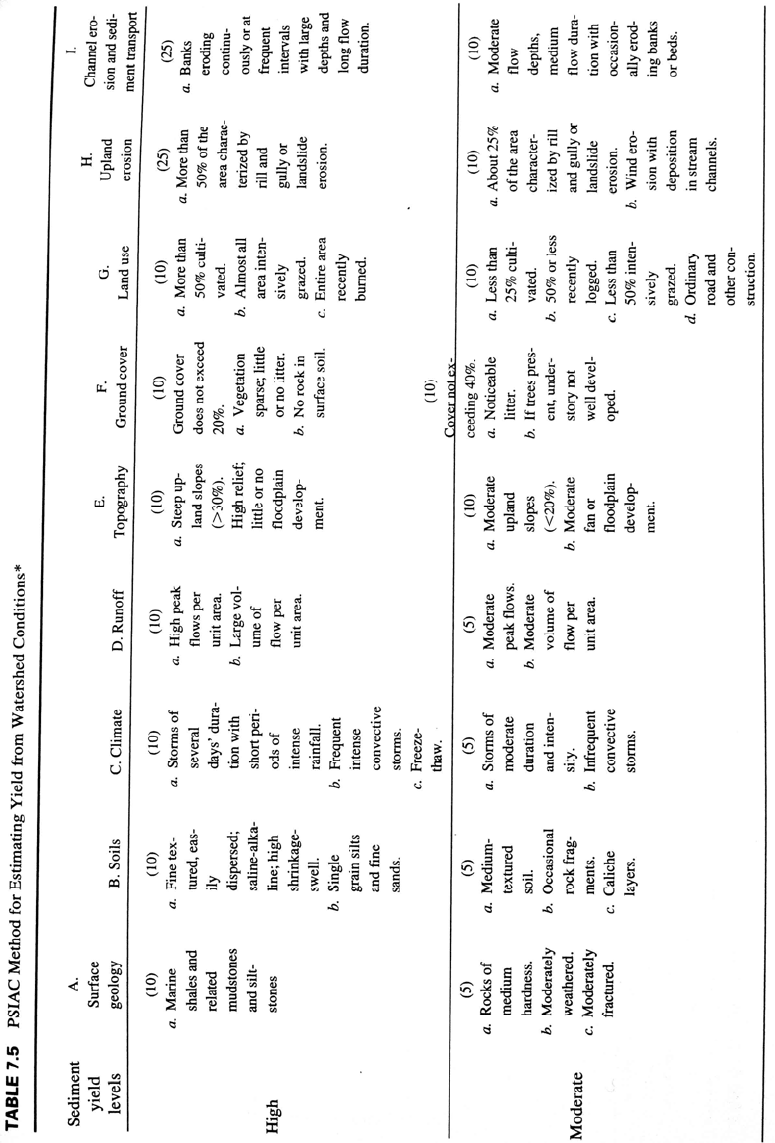
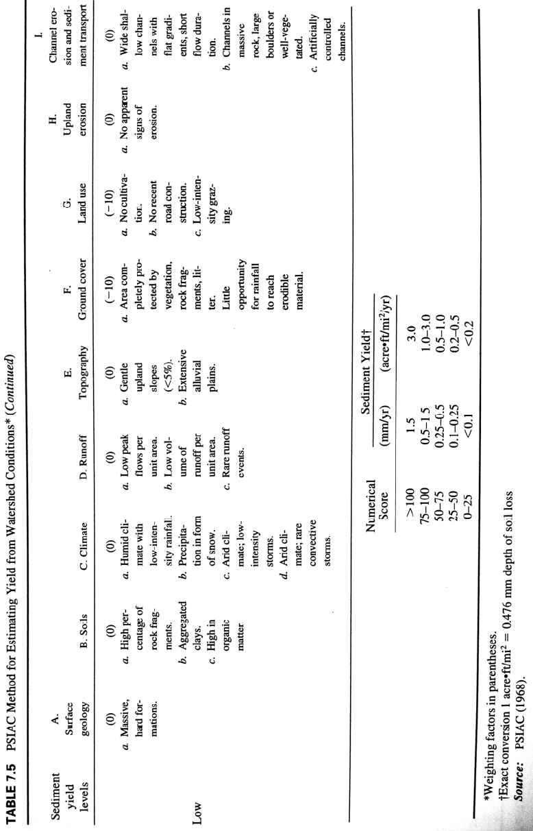
7.6.3 PSIAC Method
The Pacific Southwest Interagency Committee (PSIAC, 1968; Shown, 1970) developed a
watershed inventory method for use in the western United States to predict order-of-
magnitude sediment yields in the range of 95 to 1430 m
3
/km
2
/yr (i.e., 0.095 to 1.43
mm/yr) based on nine physical factors in the watershed. Not all of the prediction factors
are independent of one another. This method considers the yield contribution from all
types of erosion sources, and not just surface erosion as in the USLE/RUSLE type
models (Chap. 6). The methodology was tested by Shown (1970) in 28 drainage basins
between 0.05 and 96 km
2
in Colorado, Wyoming, and New Mexico for which sediment
data were available, and was found to correlate well with measured sediment yields. The
method is intended to provide rough estimates of sediment yield, and it can also be used
to determine the general magnitude of changes in sediment yield that might accompany
changes within the watershed. The rating system is summarized in Table 7.5. Other
weighting factors, or region-specific variables, may be more appropriate outside of the
western United States.
A slightly modified weighting table developed by Strand and Pemberton (1987) of the
U.S. Bureau of Reclamation is an adaptation of the PSIAC method. By personal
communication, Strand indicated that good results had been obtained with the PSIAC-
type methodology in the western United States, where it has generally provided better
results than the USLE or similar approaches which focus only on sheet erosion processes.
SEDIMENT YIELD FROM WATERSHEDS 7.33
SEDIMENT YIELD FROM WATERSHEDS 7.34
SEDIMENT YIELD FROM WATERSHEDS 7.35
Best results are obtained when the methodology is first "calibrated" by using similar
nearby basins where sediment yield is known from reservoir resurveys or extensive and
reliable stream gaging and sampling. A similar calibration approach should be used in
applying the methodology to a humid area.
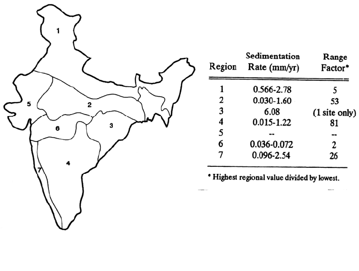
7.6.4 Sediment Yield Maps
Sediment yield mapping can undertake a variety of forms. The regionalized sediment
yield map for India (Fig. 7.22) was developed from reservoir resurvey data from 46 sites.
It illustrates the basic strategy of dividing a large heterogeneous geographic region into
subareas having presumably more uniform sediment yield characteristics. However, this
map also illustrates the problem inherent in the use of yield maps: highly variable within-
region sediment yields. Whereas the average rate of sediment accumulation between the
highest and the lowest regions in India varies by a range factor of 3, within-region
variation has a range factor as high as 81. Many factors other than regional physiography
control the rate of sediment accumulation.
Rooseboom (1992) reported on a detailed South African study to characterize and
predict sediment yield nationwide which resulted in the preparation of a sediment yield
map after other techniques failed to produce usable results. Although the approach used
in South Africa cannot eliminate the uncertainty due to yield variations that can occur
within each region, the degree of uncertainty is quantified.
The problem confronted in South Africa was that of highly variable specific sediment
yields, ranging from 1 to 880 t/km
2
/yr, including large differences even between
catchments which otherwise appeared to be nearly identical according to the available
data. There was no discernible pattern between drainage area and sediment yield. The
relatively dry temperate climate in South Africa, variety of land forms, widespread
incidence of accelerated erosion, and reduction in sediment yield in some areas due to
FIGURE 7.22 Sediment yield map for India (Shangle, 1991).
SEDIMENT YIELD FROM WATERSHEDS 7.36
upstream farm ponds and the depletion of readily erodible topsoil further complicated the
analysis. Three different methods were used to determine the sediment yield char-
acteristics of the catchments: multiple regression analysis, deterministic runoff modeling,
and regionalized statistical analysis. The analytical dataset consisted of 122 reservoirs
having between 8 and 82 years of reservoir survey data obtained by the South African
Department of Water Affairs. The following independent variables were available for the
analysis: watershed area, sediment yield, soil erodibility indices, land use, slopes, rainfall
intensity, and rainfall erosivity indices. Other parameters may also have been important
but were not available on a countrywide basis.
An attempt to develop a regression relationship was frustrated by very low levels of
significance, large standard errors of estimate, multicollinearity, and equations that
predicted negative unit yields in some cases. The second method attempted was to
construct a deterministic model describing runoff transport capacity from each catchment
and to calibrate this model against sediment yield. The rational formula was used to
determine runoff discharge, continuity and Chezy equations to convert discharge into
flow velocities and depths, and stream power to represent the sediment transport capacity
of the discharge. However, this method could not be calibrated to the dataset. Since most
of the sediment load in South African rivers is smaller than 0.2 mm in diameter, sediment
loads are dependent primarily on the amount of sediment supplied from the catchment
rather than instream transport capacity.
The third method, which was adapted, was to produce a sediment yield map by
dividing the country into nine regions judged to have relatively uniform yield potential
considering: soil types and slopes, land use, availability of recorded yield data, major
drainage boundaries, and rainfall characteristics. Regions were then further divided into
areas of high, medium, and low sediment yield potential. A constant ratio between yields
in the high-, medium-, and low-yield areas in all regions was used. The study resulted in:
(1) a national map showing nine major regions with three subregions in each; (2)
tabulated mean standardized sediment yield for each yield region; (3) graphs for each
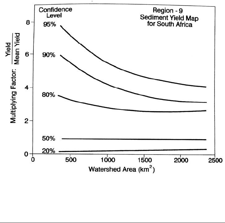
region showing the variability of yield data as a function of catchment size (Fig. 7.23);
and (4) a table giving the high, medium, and low yield potential in each region.
A four-step procedure is used to estimate sediment yield. First locate the catchment,
assign it to a region, and compute the watershed area falling within each subregion.
Second, look up the standardized regional yield from a table. Third, adjust the
standardized yield for the confidence level. For example, to conservatively estimate the
maximum expected sediment yield, enter the graph of yield variability within the region
as a function of catchment area and determine the factor at the 90 percent confidence
level (a value of 4.0 for a 1200 km
2
watershed in Fig. 7.23). Multiply the standardized
regional yield by this factor. Fourth, measure the area of the total watershed within the
high-, medium-, and low-yield modifiers and apply the subregional weighting factors to
determine the weighted average yield from the heterogeneous catchment area.
7.6.5 Erosion Modeling
Formal erosion modeling using USLE/RUSLE, WEPP (see Chap. 6), or some other
system can be used to quantify erosion and sediment yield. The fraction of the eroded
sediment delivered to the point of interest is determined by applying delivery ratios.
Properly applied, this method can provide information on both the type of erosion and its
spatial distribution across the watershed. For reliability, the results should be calibrated
against sediment yield measurements at one or more points in the study watershed.
SEDIMENT YIELD FROM WATERSHEDS 7.37
FIGURE 7.23 Variability of sediment yield as a function of catchment size within each yield area,
based on reservoir surveys (Rooseboom, 1992).
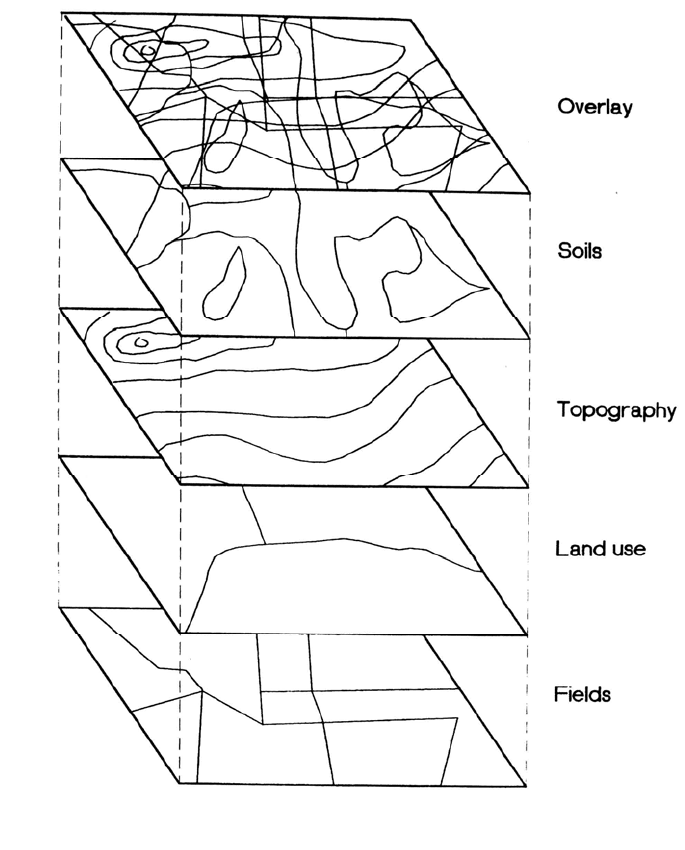
7.7 GIS AND EROSION PREDICTION
A geographic information system (GIS) is a relational database system that allows
management of multiple layers of spatially distributed information. Layers of information
can be combined, forming overlays to aid synthesis and interpretation by users (Fig. 7.24.
A GIS does not generate new data by itself, but by manipulating the database the user
may identify relationships not previously apparent. There are two types of GIS: raster (or
grid-based) systems and vector-based systems. Both types are equally powerful tools for
specific applications; they are being used for watershed management and are being linked
to erosion and hydrologic models (Shanholtz et al., 1990; Vieux and Kang, 1990).
Erosion models can be implemented in a GIS format through user interfaces or shells
written in a variety of computer languages (Lal et al., 1990; Pérez et al., 1993). The
interface allows a user to: (1) define a study area; (2) select management practices such
as crops, rotations, irrigation; (3) select soil and water conservation practices such as
contouring, terraces, and strip cropping; (4) access the GIS database to attach attributes to
model parameters; (5) execute the model and modify attribute tables; and (6) analyze and
display the results. The model spatially displays the amount of soil loss associated with
the selected management practices.
AEGIS is one of the first applications linking the crop simulation models in DSSAT1
(Tsuji et al., 1994) to a GIS. Its application in three regions in Puerto Rico is described by
SEDIMENT YIELD FROM WATERSHEDS 7.38
FIGURE 7.24 Concept of GIS overlays.
C
alixte et al. (1992), and subsequent versions of AEGIS allow the user to insert new
regions containing the required GIS layers describing soils, topography, and climate.
AEGIS has been modified and used for regional planning, such as the study conducted by
Bowen (1995) in Albania for USAID to determine fertilizer requirements for achieving
minimum wheat production targets. It is currently being applied to the southern coastal
plain of Puerto Rico to quantify the soil loss impacts of a shift from sugarcane to more-
nutrient-demanding vegetable crops that also maintain less soil cover during the growing
season and expose the soil to erosive rain. However, initial versions of AEGIS run the
former USLE model in a vector-based GIS system and predict erosion only to the edge of
the polygon. The limited ability to predict sediment delivery to channels, and subsequent
channel routing, is at present a serious limitation of GIS modeling. However, when a
downstream gage station is available, the sediment delivery can be estimated by
calibration procedures.
The LISEM model (DeRoo et al., 1994) is an example of a physically based erosion
model completely incorporated within a raster GIS system. There are no conversion rou-

SEDIMENT YIELD FROM WATERSHEDS 7.39
tines. The model is completely expressed in terms of the GIS command structure using a
prototype modeling language which allows a high level of aggregation; the entire
program code contains less than 200 lines, exclusive of comments. The processes
modeled in LISEM include interception, infiltration, splash detachment, rill and interrill
erosion, storage in microdepressions, and overland and channel flow. The results of the
model consist of GIS raster maps of soil erosion and deposition and maps of overland
flow at desired time intervals during an event.
Linkage of erosion prediction models and a GIS database containing information such
as soil erodibility, slope, land use, and climate offers the potential to examine the impacts
of management practices on erosion rates and sediment yield across large landscapes.
The potential exists to automatically analyze and predict the impacts of specific storm
tracks, including the possibility of linking with weather radar. The major theoretical
limitation with this approach is the difficulty of computing sediment delivery from each
landscape unit in the database to a downstream point of interest, such as a reservoir.
7.8 IDENTIFYING SUSPENDED-SEDIMENT SOURCES
Given the widely variable rates of sediment yield from different landscape units, erosion
control methods to reduce the inflowing load should focus on the landscape units
responsible for the delivery of most sediment to the reservoirs. Several techniques may be
used to identify sediment sources by either: (1) geographic location or (2) erosion type or
process, for example, surface erosion or channel erosion. Three basic strategies for
determining the source of suspended sediments have been outlined by Peart (1989):
indirect determination, direct measurement, and sediment fingerprinting. Sediment
sources are usually determined by indirect methods using an erosion inventory or
modeling. An erosion inventory consists only of an assessment of relative rates of erosion
and sediment delivery, without necessarily quantifying the absolute magnitude of
sediment production. Modeling, on the other hand, quantifies erosion rates within the
framework of a formal numerical methodology.
7.8.1 Indirect Determination
Methods for erosion modeling based on area-distributed models (RUSLE, WEPP) are
suitable for the indirect determination of sediment sources. These techniques have two
major limitations. First, most erosion models do not include channel erosion processes,
which must be measured and then computed separately. The second limitation is the
difficulty of assigning the sediment delivery ratio. Because the rate of surface erosion is
much larger than the sediment yield in many systems, the apportionment of sediment
loads to different source regions may depend primarily on the subjective assignment of
sediment delivery ratios to each source area. Because of these limitations, modeling of
source area contributions should be complemented with direct measurement to the
greatest extent possible.
7.8.2 Direct Measurement
Sediment production from subareas within a watershed can be directly measured by
multiple suspended sediment gaging stations. Direct measurement is an essential part of
a sediment monitoring program, especially when the watershed contains soil and land use
conditions for which erosion equations have not previously been calibrated by plot
studies, and where there is uncertainty concerning the sediment delivery ratio, as is often
SEDIMENT YIELD FROM WATERSHEDS 7.40
the case. The availability of portable, programmable sampling and data-logging
equipment incorporating pumped samplers, level recorders, turbidimeters, and tipping-
bucket rain gages makes direct measurement of sediment yield at multiple sites within a
watershed an increasingly attractive alternative. The cost of this instrumentation is very
small compared to the value of the reservoir infrastructure it is desired to protect.
As an alternative, direct measurement at selected points can be used to calibrate
regional erosion and sediment delivery models. In either case, sampling stations should
be carefully selected beforehand on the basis of, as a minimum, a preliminary assessment
of erosion sources within the watershed to identify expected high- and low-yield source
areas. A simplified erosion inventory procedure might be used for this initial assessment.
Direct measurement over an interval of years is necessary to determine rates of gully
and channel erosion. The database for soil loss measurements may be extended by using
historical air photos, historical cross-section surveys at locations such as bridge or
pipeline crossings, records of gage shift at streamgage stations, and oral histories, in
combination with current measurements and monitoring. The services of a competent
fluvial geomorphologist are highly recommended to assist evaluations of the contribution
from channel processes.
7.8.3 Qualitative Erosion Inventory
Use of a qualitative erosion inventory procedure based on field mapping to identify the
nature and spatial distribution of active sediment sources in the urbanizing 330-km
2
Anacostia watershed near Washington, D.C., was described by Coleman and Scatena
(1986). Standardized guidelines for assessing the relative importance of erosion sources
were prepared in tabular format, a sample of which is shown in Table 7.6. Four types of
land use considered to generate high sediment yields were identified: agricultural areas,
construction sites, surface mines, and stream channels. Land uses falling into these
categories, as identified from a variety of sources, were located on 1:20,000 topographic
maps. Each of 252 identified sites was then visited by a two-person inspection team to
rank sediment yield at each site as high, medium, or low compared to other land uses in
the same category, based on an assessment of both erosion rates and processes affecting
the delivery of eroded sediment to stream channels. In addition to information on the
types of problems contributing to high sediment yield, the results were also mapped to
show the spatial distribution of areas of high and low sediment yield. During inspections
the sites were also evaluated with respect to their probable future sediment load, an
important evaluation criterion because of the transitional land uses in the urbanizing basin
(recall Fig. 7.9).
7.8.4 Sediment Fingerprinting
Under favorable conditions, sediment trapped at a downstream point can be identified or
"fingerprinted" as to its source on the basis of sediment characteristics distinct to each
geographic source area or type of erosion process. Sediment characteristics may be
distinguished by geographic variations in geologic parent material or vertical variations
caused by weathering or radionuclide deposition. In the case of distinction by weathering,
the delivery of surface soil from the upper "A" horizon would be indicative of surface