Jean-Laurent Mallet. Geomodeling
Подождите немного. Документ загружается.

378
CHAPTER
8.
ELEMENTS
OF
STRUCTURAL
GEOLOGY
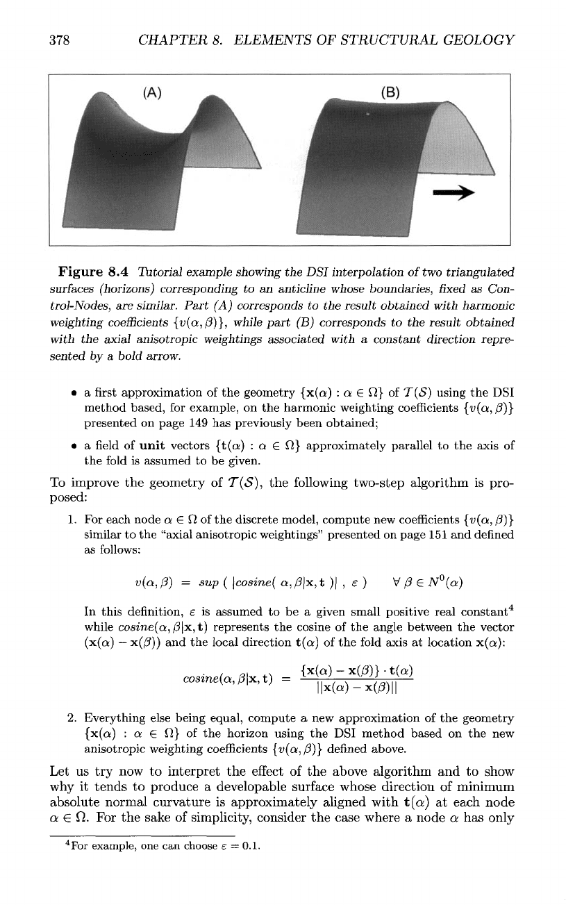
Figure
8.4
Tutorial example showing
the
DSI
interpolation
of
two
triangulated
surfaces
(horizons) corresponding
to an
anticline whose boundaries,
fixed as
Con-
trol-Nodes,
are
similar. Part
(A)
corresponds
to the
result obtained
with
harmonic
weighting
coefficients
{v(a,(3)},
while part
(B)
corresponds
to the
result obtained
with
the
axial
anisotropic weightings associated with
a
constant direction
repre-
sented
by a
bold
arrow.
• a first
approximation
of the
geometry
{x(a)
: a
(E
0}
of
T(S}
using
the DSI
method
based,
for
example,
on the
harmonic weighting
coefficients
{i>(a,/5)}
presented
on
page
149 has
previously been obtained;
• a field of
unit
vectors
{t(a)
:
a
e
17}
approximately parallel
to the
axis
of
the
fold
is
assumed
to be
given.
To
improve
the
geometry
of
T(<S),
the
following
two-step
algorithm
is
pro-
posed:
1.
For
each node
a e
17
of the
discrete model, compute
new
coefficients
{v(a,
/3)}
similar
to the
"axial anisotropic weightings" presented
on
page
151 and
defined
as
follows:
In
this
definition,
e is
assumed
to be a
given small positive real
constant
4
while
cosine(a,/3
x, t)
represents
the
cosine
of the
angle between
the
vector
(x(a)
—
x(/3))
and the
local direction
t(a)
of the
fold
axis
at
location
x(a):
2.
Everything else being equal, compute
a new
approximation
of the
geometry
(x(a)
: a e 17} of the
horizon using
the DSI
method based
on the new
anisotropic
weighting
coefficients
{v(a,(3)}
defined
above.
Let
us try now to
interpret
the
effect
of the
above
algorithm
and to
show
why
it
tends
to
produce
a
developable
surface
whose
direction
of
minimum
absolute
normal
curvature
is
approximately
aligned
with
t(a)
at
each
node
a G
0.
For the
sake
of
simplicity,
consider
the
case
where
a
node
a has
only
4
For
example,
one can
choose
e —
0.1.
8.2.
MODELING STRATIFIED MEDIA
379
four
neighbors
/3^,
(3^
,
^,
and
/?Q~
whose
locations
after
step
1 of the
above
algorithm
are
assumed
to be
such
that
Such
an
initial geometry
will
generate
the
following
anisotropic weighting
coefficients
{v(a,/3)}
at
step
1 of the
above algorithm:
At
step
2 of the
above algorithm, using these anisotropc weightings
and
min-
imizing
the
DSI
local roughness
R(x\a)
will
tend
to
move
the
node
a to the
center
of
gravity
of its
neighbors
/?f
and
j3^.
Consequently,
the
nodes
a,
/3f,
and
J3^
tend
to
become aligned,
and the
normal curvature
in the
direction
t(ct)
tends
to
vanish.
In
practice,
it can be
observed
that
the
direction
of
absolute minimum curvature tends
to
become aligned with
t(o:);
this implies
that
the
Gaussian curvature
K at
node
a
will also tend
to
vanish.
As a
con-
sequence, according
to the
property
(5.58),
the
surface will tend
to
become
developable.
A
tutorial
example
Figures
(8.4)-A
and
(8.4)-B
show
a
tutorial example where
a
surface
is
con-
strained only
by
Control-Nodes located
on its
boundary. Using
the DSI
algo-
rithm based
on the
harmonic weightings
{v(a,(3}}
generates
the
surface (A).
If
the
axis
of the
fold
is
specified
(bold
arrow),
then
the
cosine weightings gen-
erate
the
surface
(B)
whose shape
is
more acceptable
than
(A) for a
geological
anticline.
8.2
Modeling
stratified
media
As
suggested
in
figure
(8.5),
the
exploration
of
sedimentary stratified struc-
tures
in the
subsurface
is
based
on two
sources
of
information:
• the
seismic
data,
which
are
used
to
observe
and
model
the
main
horizons
bounding
"macro
layers";
• the
well-markers,
which
allow
us to
identify
the
presence
of
internal
horizons
not
actually
"seen"
on the
seismic
images
and
splitting
the
macro
layers
into
"micro
layers."
Assuming
that
the top and
bottom
horizons
5
of a
macro layer
are
given,
this
section addresses
the
problem
of
building
the
internal horizons corresponding
to a
series
of
well-markers.
For
this purpose,
a
solution based
on a
"morphing"
technique (see [32,
121])
coupled with
DSI is
proposed.
5
The top and
bottom
horizons
of a
layer
are
also called
the
"hanging-wall"
and
"foot-
wall"
of the
layer,
respectively.
380
CHAPTER
8.
ELEMENTS
OF
STRUCTURAL GEOLOGY
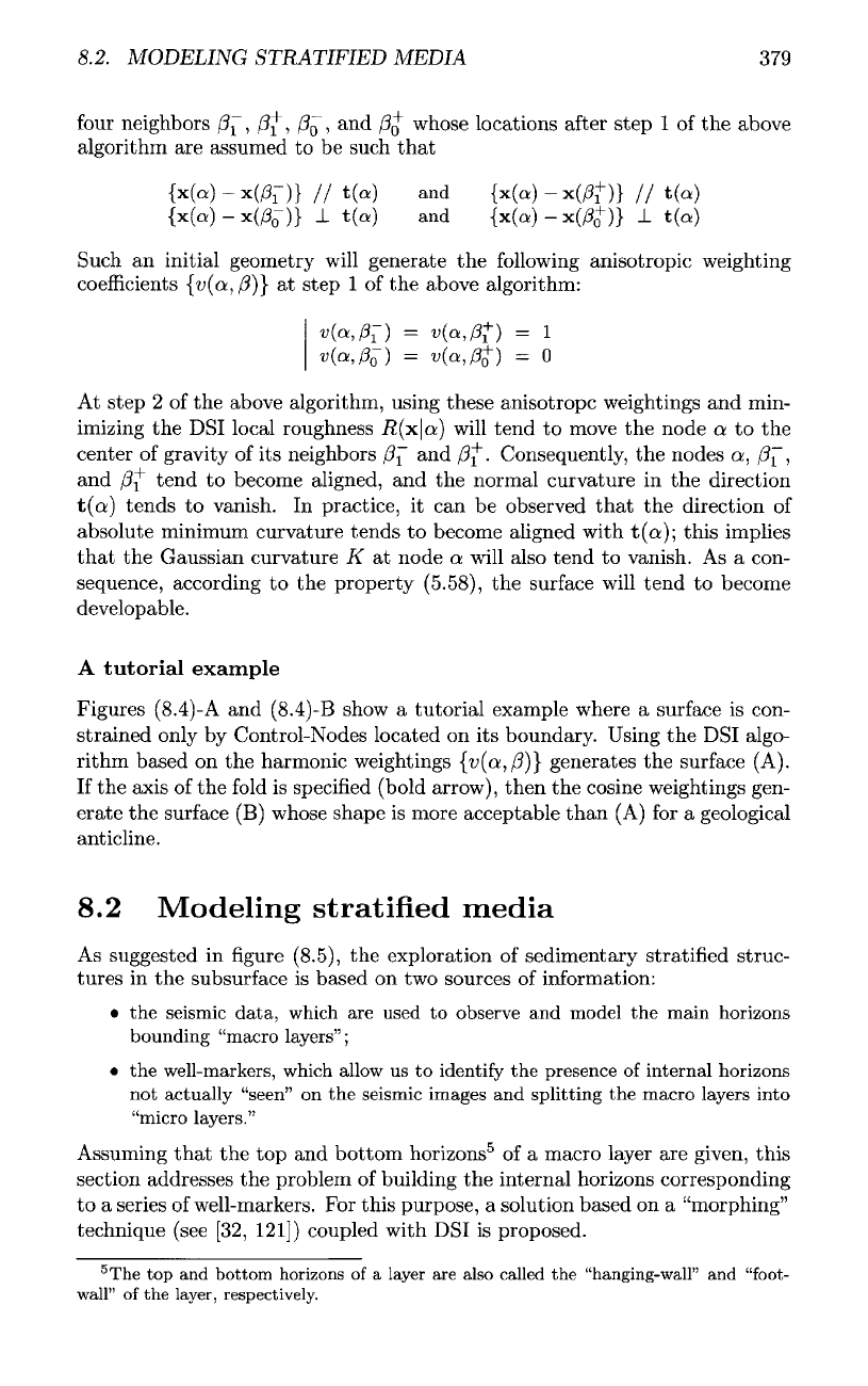
Figure
8.5
Cross
section
of a
"macro"
layer
bounded
by two
horizons
SQ
and
Si
(bold
lines)
actually
"seen"on
the
seismic
images
and
containing
a
series
of
internal
horizons
{Si}
(white
lines)
identified
by
well-markers
(white
points)
that
correspond
to the
intersection
of
the
wells
with
these
intermediary
horizons.
"Ghost"
well-markers
that
correspond
to
points
of
the
well-paths
not
intersecting
an
internal
horizon
are
represented
as
black
points.
8.2.1
Simple morphing
In
computer science literature (e.g,
see
[121]),
any
continuous transformation
of
a
"source" object
OQ
into
a
"target"
object
O\
is
called
a
"morphing"
or
a
"metamorphosis."
For
example,
let us
assume
that
the
source object
OQ
=
T(«So)
is a
triangulated
surface
whose geometry
is
represented
by a
discrete model
.M
3
(O,
N,
x
0
,Cx
0
)
and
which
has to be
transformed into
a
given
target
surface
6
Si.
Such morphing requires building
a
vectorial
function
m
defined
on
Q
such
that
The
vectorial
function
m so
defined
is
called
a
"morphing"
function
and can
be
represented
by a
discrete model
A4
3
(fi,
TV,
m, Cm)
based
on the
same graph
G(M,N)
as the
geometry
of
T(«S
0
).
In
practice,
as
suggested
in figures
(8.6)
and
(8.7),
the
morphing function
m is
built
as
follows:
• For
each node
at,
e
fJ
belonging
to the
boundary
of
T(<So):
—
determine,
on
<Si,
the
point
y(ctb)
"geologically
associated"
with
x(at,)
such
that
y(ctb)
should
be
equal
to
(xo(ab)
+
m(o!6));
—
add to Cm a
control-vector
7
specifying
that
m(a&)
should
be
equal
to
(y(ab)-xo(orb)).
6
Note
that
Si
does
not
have
to be a
triangulated
surface.
7
If
need
be, it is
also
possible
to add
control-vectors
m not
located
on the
boundary
of
SQ
and
joining
an
internal
point
of
SQ
to a
point
on
Si.
8.2.
MODELING STRATIFIED MEDIA
381
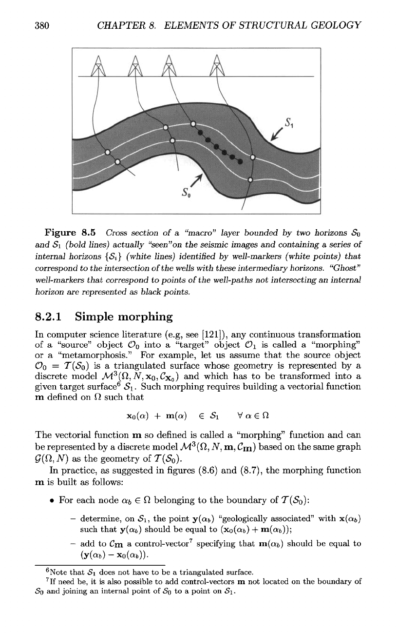
Figure
8.6
Cross
section
showing
how
morphing
vectors
attached
to the
nodes
of
T(So)
bridge
the top and
bottom
surfaces
(Si)
and
(So)
of
a
layer.
The
morphing
vectors
bridging
the
boundaries
or
tangent
to the
fault
traces
are
assumed
to be
given
and
set as
"control-vectors"
(bold
vectors),
while
the
other
vectors
are
continuously
interpolated
using
DSL A
well-marker
(white
point)
is
projected
onto (So)
(black
point)
in the
opposite
direction
to
that
of
the
morphing
vectors.
•
Interpolate
m
with
DSI;
as a
consequence,
all the
points
as
defined
by
(x
0
(a)
+
m(o!))
will
be
approximately
located
on
Si
for any a
e
Q.
•
Apply postprocessing
to m so
that
all the
points
(xo(a)
+
m(a))
get
strictly
located
on
Si
for any a
G
Jl.
The
morphing function
m so
defined
can be
used
to
build
a
family
of
trian-
gulated surfaces
{T(St)
:
t
G
[0,1]}
having
a
geometry
x
t
,
as
defined
by
As
shown
in figure
(8.5),
these surfaces split
the
layer bounded
by the two
initial
surfaces
SQ
and
Si
in a
"proportional" stratigraphic
style.
8
8.2.2
Generalized morphing
In
addition
to the
discrete models
_M
3
(0,
N,
xo,Cx
0
)
and
M^(£l,
TV,
m,C
m
)
introduced above,
let us
consider
a
third discrete model
M
n
($l,
N,
p,C
v
)
where
(p
is an
n-dimensional
vectorial
function
called
a
"relative thickness
function"
and
defined
at the
same nodes
as
x
0
and m:
8
Traditionally,
there
are
three
main
styles:
on-lap,
off-lap,
and
proportional.
382
CHAPTER
8.
ELEMENTS
OF
STRUCTURAL GEOLOGY
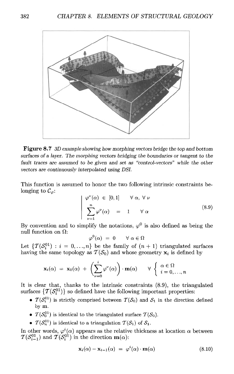
Figure
8.7
3D
example showing
how
morphing vectors bridge
the top and
bottom
surfaces
of
a
layer.
The
morphing vectors bridging
the
boundaries
or
tangent
to the
fault
traces
are
assumed
to be
given
and set as
"control-vectors" while
the
other
vectors
are
continuously interpolated using
DSL
This
function
is
assumed
to
honor
the two
following
intrinsic constraints
be-
longing
to
C
v
:
By
convention
and to
simplify
the
notations,
<p°
is
also
defined
as
being
the
null
function
on
J7:
Let
{T(Sf
l
)
:
i — 0,
...,n}
be the
family
of
(n
+ 1)
triangulated
surfaces
having
the
same topology
as
T(<So)
and
whose geometry
x^
is
defined
by
It is
clear
that,
thanks
to the
intrinsic constraints
(8.9),
the
triangulated
surfaces
(T(<S?
1
)}
so
defined
have
the
following
important properties:
•
T(Sf
l
)
is
strictly comprised between
T(<So)
and
<Si
in the
direction defined
by
m.
•
T(»So
1
)
is
identical
to the
triangulated surface
T(<So).
•
T(<S°
1
)
is
identical
to a
triangulation
T(iSi)
of
Si.
In
other words,
(p
l
(o)
appears
as the
relative thickness
at
location
a
between
T(Sfl
l
]
and
T^S?
1
)
in the
direction
m(a):
8.2.
MODELING STRATIFIED MEDIA
383
Equation (8.10) suggests
that
(f>(ot)
can be
used
for
modeling both
the
local
variations
of the
thickness
and the
stratification style
of a
series
of n
micro
layers inside
a
macro layer bounded
by
T(So)
and
S(S\).
Prom
a
DSI
point
of
view,
it can be
observed
that
the
intrinsic constraints
(8.9)
to be
honored
by the
relative
thickness
function
(p
are
identical
in
form
to the
intrinsic constraints (10.8) presented
on
page
540 for
controlling
the
behavior
of
Membership Functions.
8.2.3
Fitting
well-markers
Let us
imagine
that
the
internal horizons
{T(Sf
l
)
:
i =
1,...,
(n
—
1)}
defined
above have
to fit a
series
of
markers observed
on
wells
and
consisting
of
points
IP
z
fc
(f)
such
that
9
IP*CO
=
Ah
intersection
of
T(S°
l
)
with
the
well
W
fc
As
suggested
in figure
(8.6),
for
each well-marker
IPf
(f),
it is
always possible
to find a
point
pf(^)
in a
triangle
T =
T(x
0
(ao),x
0
(ai),xo(a;2))
of
T(«S
0
)
such
that
•
pf(£)
has
local
barycentric
coordinates
10
(u,v)
in T:
•
pf(£)
is the
projection
of
IP^(^)
onto
T(«So)
in the
direction
mr(u,v),
as
denned
by
Let
<^T(U,V)
be the
local linear interpolation
of
(p
on T, as
defined
by
For
T(S®
1
}
to
pass
by
IPf
(£),
the
local interpolation
(pr(u,
v]
of
(p
on T
must
honor
the
following
constraint:
This constraint
is
equivalent
to the DSI
constraint
c,
which depends
on the
following
parameters
9
Note
that
the
same
well
can
intersect
the
same
internal
horizon
several
times.
10
See
definition
(6.15).
384
CHAPTER
8.
ELEMENTS
OF
STRUCTURAL GEOLOGY
and as
defined
by
where
a
c
is a
normalizing factor,
as
defined
by
Let us
define
9
c
((p)
as
follows:
When added
to the set of
constraints
C^
of the
discrete model
M
n
(fi,
JV,
</?,
C
v
},
for
each
v
<
i,
this
constraint
induces
terms
7^
(a) and
r^(a|(/?)
in the
local
form
of the
DSI
equation such
that
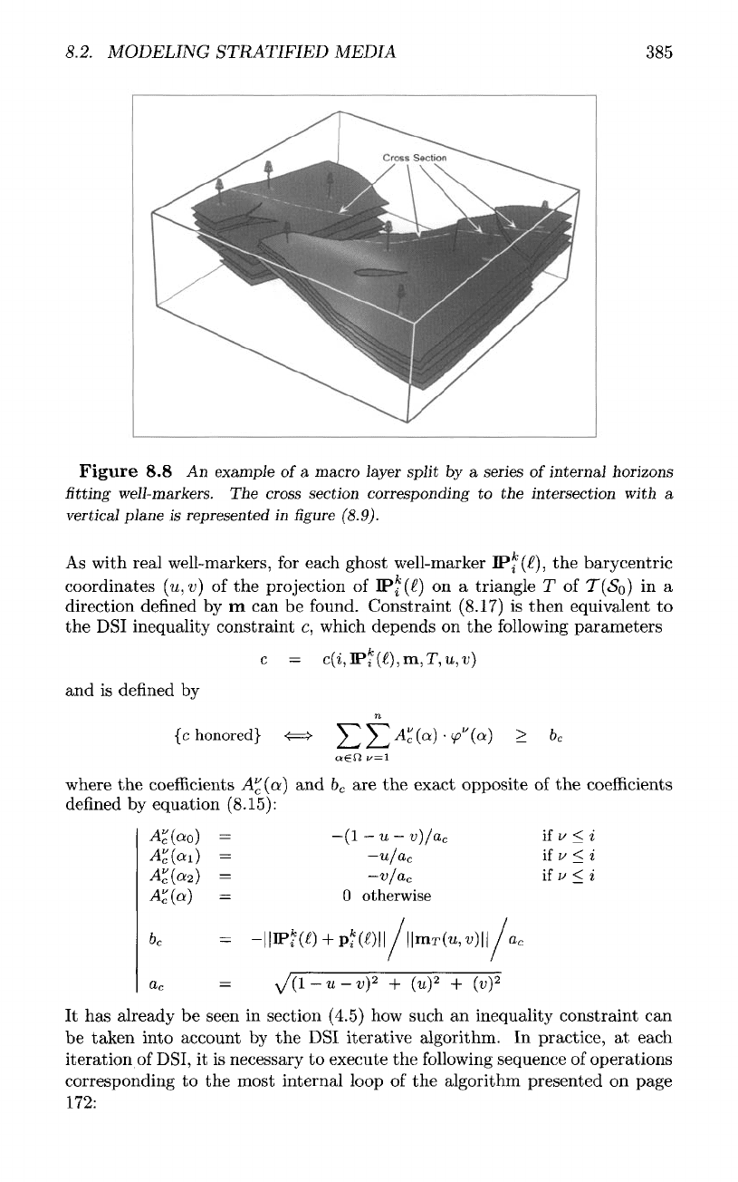
Figure (8.8) gives
a
real case example
of the
application
of the
method
de-
scribed
above.
8.2.4
Fitting
ghost
well-markers
In
the
case
of a
reservoir bounded
by the top and
bottom horizons
T(«Si)
and
«So,
a
well
W
fc
may not
intersect
a
given internal horizon
T(»S°
1
).
Such
an
event
can be
interpreted
as a
piece
of
information
on the
position
of
T(Sf
l
)
relative
to
W
fc
:
in the
direction
(—m),
the
horizon
T(<Sf
l
)
is
"below"
all the
points
on the
path
of
W
fc
.
To
take this kind
of
information into account,
the following
procedure
is
proposed:
1.
As
suggested
in figure
(8.5),
build
a
series
of
"ghost"
well-markers
(IP^^)
:
I
—
1,2,...}
corresponding
to a
regular
sampling
of the
path
of
W
k
.
2.
For
each
ghost
well-marker
IPf
(i),
introduce
an
inequality
constraint
on the
relative
thickness
function
specifying
that
8.2.
MODELING STRATIFIED MEDIA
385
Figure
8.8 An
example
of
a
macro
layer
split
by a
series
of
internal
horizons
fitting
well-markers.
The
cross
section
corresponding
to the
intersection
with
a
vertical
plane
is
represented
in figure
(8.9).
As
with real well-markers,
for
each ghost well-marker
JP
i
(^),
the
barycentric
coordinates
(u,
v)
of the
projection
of
IP^
(I)
on a
triangle
T of
T(So]
in a
direction
defined
by m can be
found.
Constraint (8.17)
is
then equivalent
to
the
DSI
inequality constraint
c,
which depends
on the
following
parameters
and is
defined
by
where
the
coefficients
A"
(a) and
b
c
are the
exact
opposite
of the
coefficients
defined
by
equation
(8.15):
It has
already
be
seen
in
section (4.5)
how
such
an
inequality constraint
can
be
taken
into
account
by the DSI
iterative
algorithm.
In
practice,
at
each
iteration
of
DSI,
it is
necessary
to
execute
the
following
sequence
of
operations
corresponding
to the
most internal loop
of the
algorithm presented
on
page
172:
386
CHAPTER
8.
ELEMENTS
OF
STRUCTURAL GEOLOGY
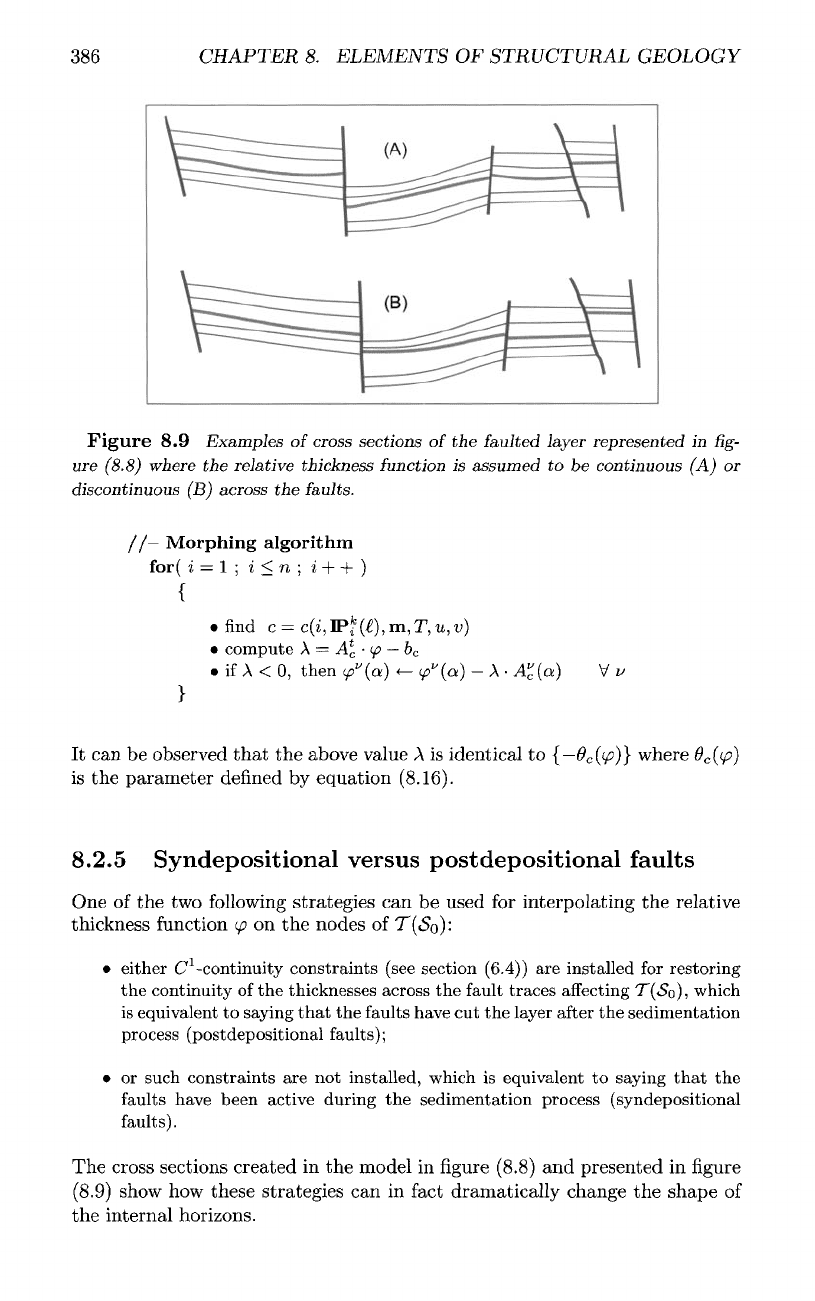
Figure
8.9
Examples
of
cross sections
of the
faulted
layer
represented
in fig-
ure
(8.8) where
the
relative thickness function
is
assumed
to be
continuous
(A) or
discontinuous
(B)
across
the
faults.
/
/-
Morphing
algorithm
for(
i = I
;
i
<
n ; i + + )
{
• find c =
c(i,~S>i(l},m,T,u,v]
•
compute
A
=
A*
c
•
tp
—
b
c
• if A < 0,
then
</?"(a)
<-
^"(a)
- A •
A
v
c
(o)
V
v
}
It can be
observed that
the
above
value
A is
identical
to
{—O
c
((p)}
where
O
c
((p)
is
the
parameter
defined
by
equation
(8.16).
8.2.5
Syndepositional
versus
postdepositional
faults
One
of the two
following
strategies
can be
used
for
interpolating
the
relative
thickness
function
(p
on the
nodes
of
T(<$o)
:
•
either
C
1
-continuity
constraints
(see
section
(6.4))
are
installed
for
restoring
the
continuity
of the
thicknesses across
the
fault traces
affecting
T(«So),
which
is
equivalent
to
saying
that
the
faults have
cut the
layer
after
the
sedimentation
process
(postdepositional
faults);
• or
such constraints
are not
installed, which
is
equivalent
to
saying
that
the
faults
have been active during
the
sedimentation process (syndepositional
faults).
The
cross
sections
created
in the
model
in
figure
(8.8)
and
presented
in figure
(8.9)
show
how
these strategies
can in
fact
dramatically change
the
shape
of
the
internal
horizons.
8.2.
MODELING STRATIFIED MEDIA
387
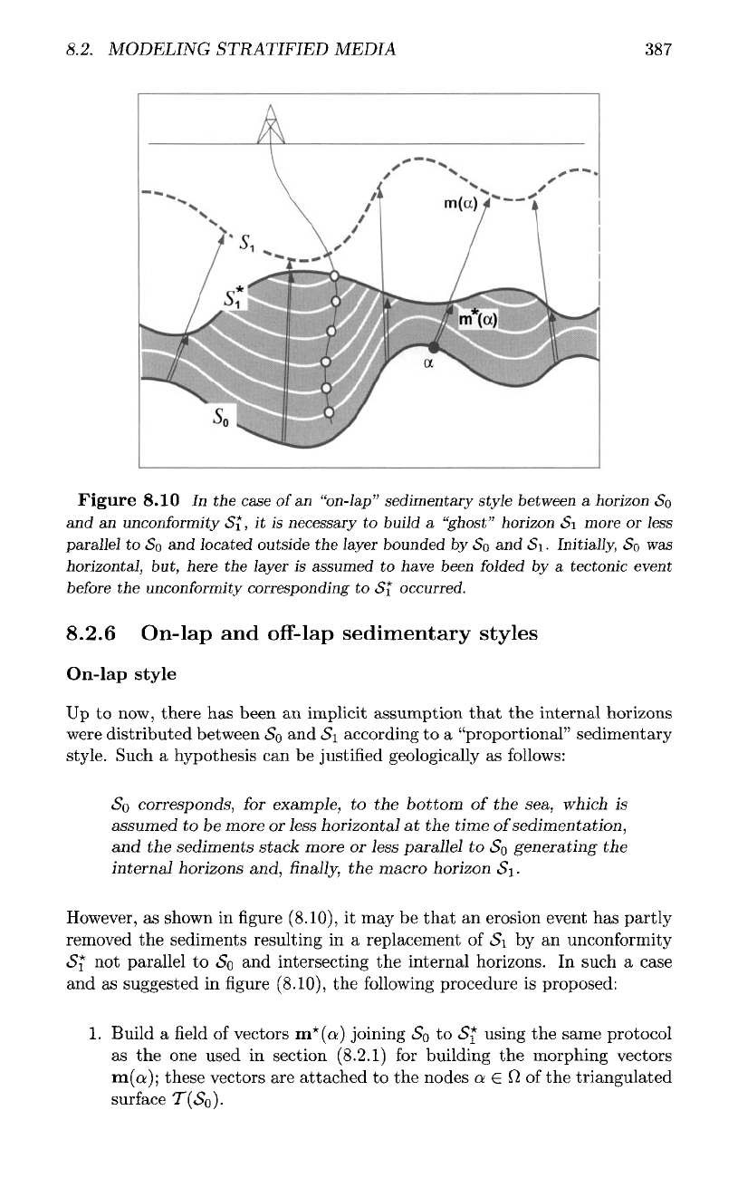
Figure
8.10
In the
case
of
an
"on-lap"
sedimentary
style
between
a
horizon
SQ
and
an
unconformity
Si,
it is
necessary
to
build
a
"ghost"
horizon
<Si
more
or
less
parallel
to So and
located
outside
the
layer
bounded
by So and
Si.
Initially,
So was
horizontal,
but,
here
the
layer
is
assumed
to
have
been
folded
by a
tectonic
event
before
the
unconformity
corresponding
to
Si
occurred.
8.2.6
On-lap
and
off-lap
sedimentary
styles
On-lap
style
Up
to
now,
there
has
been
an
implicit assumption
that
the
internal horizons
were
distributed between
SQ
and
Si
according
to a
"proportional" sedimentary
style. Such
a
hypothesis
can be
justified
geologically
as
follows:
SQ
corresponds,
for
example,
to the
bottom
of the
sea, which
is
assumed
to be
more
or
less horizontal
at the
time
of
sedimentation,
and
the
sediments stack more
or
less parallel
to
SQ
generating
the
internal horizons and,
finally, the
macro horizon
Si.
However,
as
shown
in figure
(8.10),
it may be
that
an
erosion event
has
partly
removed
the
sediments resulting
in a
replacement
of
Si
by an
unconformity
S^
not
parallel
to SQ and
intersecting
the
internal horizons.
In
such
a
case
and as
suggested
in figure
(8.10),
the
following
procedure
is
proposed:
1.
Build
a field of
vectors
m*(o:)
joining
SQ to
S*
using
the
same protocol
as the one
used
in
section
(8.2.1)
for
building
the
morphing vectors
m(a);
these vectors
are
attached
to the
nodes
a
e
0 of the
triangulated
surface
T(«$o).