Ellis,J. Pressure transients in water engineering, A guide to analysis and interpretation of behaviour
Подождите немного. Документ загружается.

A number of options exists as far as choosing the representative set of
characteristics. Several of these will be described with the advantages
and disadvantages of each mentioned.
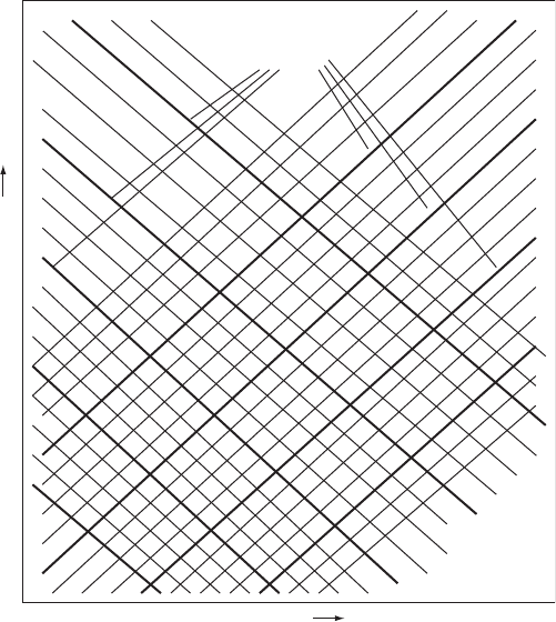
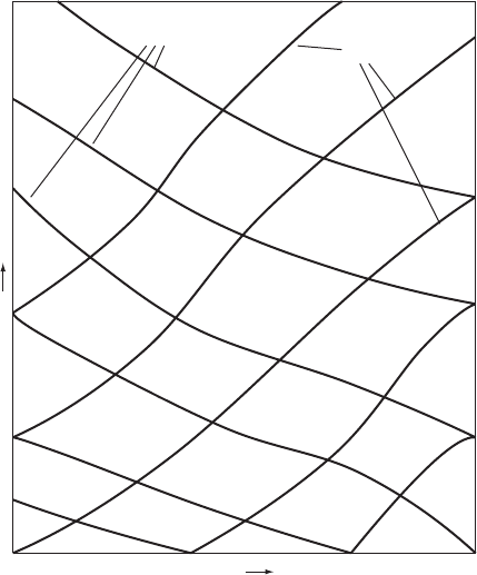
5.2 ‘Natural’ characteristic mesh
An initial set of paths is chosen and the progress of these followed as
time passes (Fig. 5.4). The intersection points of opposing paths
provide solutions for transient flow conditions. Values obtained are
accurate and this approach has the capability of detecting shock
fronts and to follow their progress. While a regular distribution of
characteristics may be chosen at the outset, as time passes the distribu-
tion of intersection points at which solutions are found becomes
increasingly irregular, particularly where appreciable variations in
wave speed occur as when gas release takes place. For a simple pipeline
having uniform properties along its length, this method poses no
52
Representative characteristics
+
t
+
x
C– C+
Fig. 5.3. Representative characteristics in the x—t plane
Pressure transients in water engineering
significant difficulties and has been used effectively by Larsen (1976) for
example, in his investigation of undersea outfalls. Considerable
complexity is introduced where a looped or branching system is
encountered or where internal changes of pipe material or diameter
are present for instance. Although not insurmountable, the computa-
tional difficulties of following progress of characteristics through more
complicated systems are sufficient to make this approach unattractive
for general use.
The irregular distribution of intersection points at which solutions
are obtained also means that some post-processing is required to
make the predictions easy to understand. Typically the end-user
wishes to see time variations of pressure, head, flow, etc., at specified
locations and this requires interpolation within the irregular mesh of
solutions.
Almost all computational schemes designed for general use employ a
regular or ‘fixed’ mesh arrangement which provides predictions at
predefined locations throughout the pipeline system and at regular
increments of time. Characteristic paths are selected, from the 1
53
+x
C– paths
C+ paths
+t
Fig. 5.4. ‘Natural’ or irregular characteristic mesh
Application of characteristic equations
available in each direction, which intersect at the predefined mesh
points. There remain considerable differences between alternative
fixed-mesh schemes with much of the difference centred on how the
wave speed is handled.
5.3 Using variable wave speed a
The equation for acoustic velocity or wave speed a has been given in
Chapter 3 as:
a ¼ 1=
p
f
m
ðDc
1
=ðsEÞþð1 Þ=K þ =ðp
abs
Þg ð3:7Þ
where
m
¼ð1 Þ þ
g
.
The wavespeed given by equation (3.7) is a composite involving
three components: the solid pipe or tunnel wall, the liquid component
and the gaseous component. Variability of the wave speed with chan-
ging pressure for a given gas content produces changes in characteristic
gradients dx=dt ¼ V a.
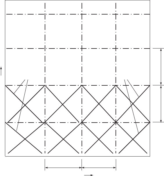
Use of a fixed grid as shown in Fig. 5.5 allows computation to be
carried out in a way that yields values of the dependent variables flow
rate, pressure and gas content at regular intervals along each pipeline
of a system and at fixed time intervals. As the wave speed changes
with pressure during a transient event, especially at low pressure,
then the gradients:
dx=dt ¼ V a
will alter and it is necessary to interpolate on the previous time line to
establish values for the Riemann quasi-invariants. The solution can
then be obtained at the intersection points of opposing pairs of charac-
teristics. Most schemes rely on the interpolation points being within the
pipeline sections directly on each side of the solution point. This
requires that the distance increment x and the time increment t
be chosen so that the quotient:
x=t jV aj
max
ð5:3Þ
This Courant Lewy stability criterion ensures that interpolation takes
place between the adjacent grid points. Any appreciable and continued
extrapolation beyond these grid points is likely to lead to instability. The
interpolation point should lie as close to the grid point as possible but
without falling outside the reach of the pipeline. Fox (1977) describes
use of such a scheme and, based upon experience, has found that
x=t ¼ a=0:95 works well. The process of interpolation leads to
54
Pressure transients in water engineering
some dispersion of the wave front and there is an element of compro-
mise involved between minimising the effects of numerical dispersion
while retaining the ability to model variable wave speed.
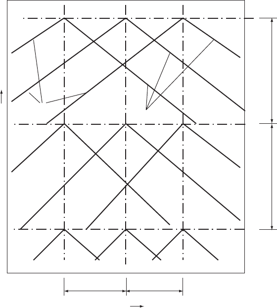
5.4 Use of a larger time step
A numerical approach which can permit smaller quotients or effectively
larger time steps t for the same x increments:
x=t < jV ajð5:4Þ
was described by Vardy (1976). This involves a more complicated
routine to identify the position of the interpolation point as shown in
Fig. 5.6. While not restricted to variable wave speed schemes, this
approach can retain the ability to accommodate variable speed of
55
+x
C– characteristics
dx/dt = V – a
C+ characteristics
dx/dt = V + a
Dx
D
t
D
t
Dx
+t
Fig. 5.5. Fixed-grid characteristic mesh
Application of characteristic equations
propagation of the pressure waves but contains the same risks of disper-
sion of the wave front.
5.5 Use of a fixed wave speed
Streeter and Wylie (1967) used a different approach. The effect of
velocity upon the characteristic gradient dx=dt was neglected, and a
was taken as constant, giving:
dx=dt ¼a ð5:5Þ
By setting:
x=t ¼ dx=dt ¼ constant
56
+
x
Dx Dx
D
t
D
t
C+ characteristics
C– characteristics
+
t
Fig. 5.6. Fixed-grid mesh with extended time steps
Pressure transients in water engineering
the need for interpolation is avoided and with it the effects of any
numerical dispersion.
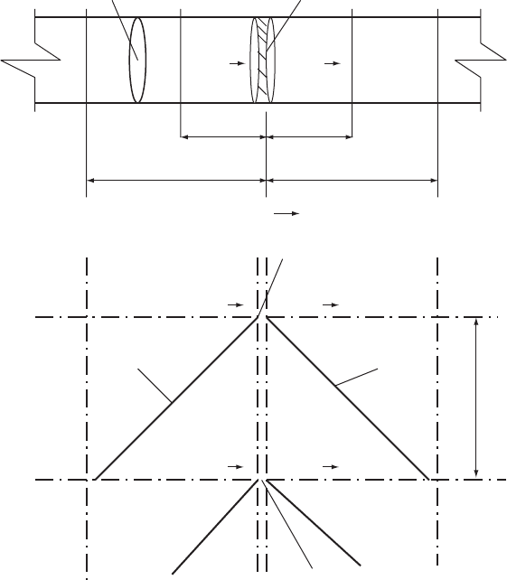
In this scheme, free air or gas released from solution, which can influ-
ence the wavespeed a, is handled by ‘collecting’ all of the gas in the
neighbourhood of a computing point, into a single ‘bubble’ occupying
the cross-section of the pipe at a local computing point (Fig. 5.7). A
discontinuity of velocity (and flow) occurs across the bubble which
expands and contracts as pressure changes. Behaviour of the gas mass
is represented using a gas law.
If the gas void fraction in the neighbourhood of a solution point and
at the start of a time increment t is
o
at absolute pressure p
absðoÞ
and
57
Cross-sectional area = A Gas volume = aADx
Initial volume = a
1
ADxh
atm
/h
abs(o)
C+ characteristic C– characteristic
Final volume = (a
1
+ a
f
)ADxh
atm
/h
abs
+
x
Dx/2
V
u/s
V
d/s
Dx/2
V
u/s
V
d/s
V
u/s(o)
V
d/s(o)
Dx
Dt
Dx
Fig. 5.7. Representation of free gas in fixed-grid computations
Application of characteristic equations

it is assumed that this fraction is representative of
1
2
x on each side of
the solution point then the total gas volume at the solution point will be
0
xA cubic metres.
The following equations are available to provide values of upstream
and downstream velocities V
u=s
and V
d=s
, piezometric level H and
final void fraction at the end of the time increment.
From the advancing Cþ characteristic, Jþ¼V
u=s
þ g=aH and from
the backward C characteristic, J¼V
d=s
g=aH from conservation
of volume across the bubble over the time increment,
fV
d=s
þ V
d=sðoÞ
ðV
u=s
þ V
u=sðoÞ
ÞgA=2 ¼ A x d=dt ð5:6Þ
where void fraction is given by:
¼ð
1
þ
f
Þh
atm
=h
abs
d=dt ¼ h
atm
dð
1
=h
abs
Þ=dt þ h
atm
dð
f
=h
abs
Þ=dt
if free gas content is
o
at the start of the increment then,
h
atm
dð
1
=h
abs
Þ=dt h
atm
o
ð1=h
2
abs
ÞðH H
o
Þ=t
and
h
atm
dð
f
=h
abs
Þ=dt h
atm
=h
abs
d
f
=dt
where the derivative d
f
=dt is the rate at which gas is evolving from
solution. This is a quantity that can range from all available gas being
freed as used by Fox (1977) to a more controlled rate of release. The
relationship between piezometric level or total head H and the absolute
pressure head h
abs
is:
h
abs
¼ H z þ h
atm
These equations are sufficient to provide solutions for the flow variables
at the close of the time increment.
This approach avoids the need for interpolation and thus any risk of
numerical dispersion. However, even where interpolation is used, this is
mainly significant only at low pressures when gas bubbles are forming,
with pressure changes being modest so that any errors introduced to
interpolation are not likely to be very significant.
5.6 Distribution of free gas along the pipeline
Other implementations of the equations have also used the fixed
regular grid but handled the matter of wave speed and gas release in
different ways. For example, a constant wave speed is maintained in
58
Pressure transients in water engineering
each pipe, based upon the composite pipe and liquid system. Gas release
is modelled as a separate phase which may be either distributed along
the top of the pipe in the form of a continuous gaseous phase, or
could be represented as a discrete bubble where it occurs at a well-
defined summit on the pipeline. A flexible model will include the
option of representing free gas or vapour in one or both of these forms.
5.7 Model output
Nowadays, rarely does the user require to consider the detailed schema-
tisation of a pipeline or the relationship between x and t. These
aspects will often be resolved by the computer program itself.
Using one of the approaches described in sections 5.3 to 5.6, values of
head H, pressure ¼ gðH zÞ, velocity V and flow rate can be
predicted at each of the intersection points of the characteristics. For
each simulation this process is continued until all significant effects
have been modelled. It is then a relatively straightforward matter to
present these predicted values in forms which are readily understood.
Both tabular and graphical presentations are considered important.
Plotted output usually can take two forms. First, time histories of
specific variables such as flow, pressure or air volume at defined loca-
tions within a network for instance, allow timescales of events to be
easily identified and the changes at one place to be related to
changes at other points. Amplitude of pressure transient oscillations
can also be seen in these plots. The second form of graphical presenta-
tion is ‘envelope’ curves showing the variation of extremes of head or
pressure, for example, throughout a pipeline. This type of plot allows
the engineer to identify zones of sub-atmospheric pressure or regions
where peak pressure has exceeded allowable limits.
Tabulated information on extremes of pressure and flow avoids the
need to scale information from graphical output and complements
the plotted forms of presentation.
59
Application of characteristic equations
6
Boundaries
In earlier chapters it was described how the task of determining flow and
pressure changes along a pipeline could be achieved by using the
network of characteristics and the values propagating along these
paths. The challenge remains of finding corresponding values of flow
parameters at the many and various features and fittings which are to
be found in most pipeline networks. Each feature will act to transmit
and/or reflect transient pressure waves in a manner which is particular
to that type of fitting or element of the pipeline. Each of these elements
is referred to as a boundary. Analysis of response of these features
requires that an additional ‘auxiliary’ equation or equations has to be
introduced to complete the process of solution and this chapter intro-
duces just some of the wide variety of possible pipeline elements and
the corresponding equations.
At each computing point within a pipeline, values of velocity V and
total head H were obtained through solving a pair of simultaneous equa-
tions at the intersection point of characteristics travelling in opposing
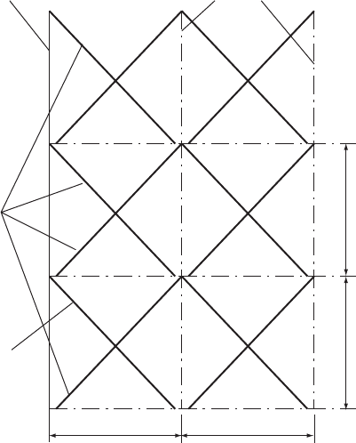
directions within the pipeline. At the upstream and downstream extremi-
ties of a pipeline only a single characteristic intersects the boundary at any
instant of time, as shown in Fig. 6.1. Since values of both V and H are
required it is necessary to introduce additional equation(s), sometimes
referred to as auxiliary equations, to provide a complete description of
conditions at the extremity of the pipeline. The nature of boundaries is
varied and it is worthwhile spending a little time in considering some
of the types and common assumptions which are made regarding these.
As a rule the steady flow characteristics of a boundary such as a valve
or pump are assumed applicable to unsteady conditions.
Boundaries usually represent some actual physical feature of a
network but may also be numerical devices introduced for convenience
60
or to simplify computations. Examples of both types are presented in
this chapter. While some boundaries occur at the physical extremities
of pipelines such as where a pipeline discharges to a tank or reservoir,
others may occur partway along a main. Such internal boundaries can
include in-line valves, booster pumps and self-acting air valves and
pressure relief valves.
6.1 Types of boundary
It is at boundaries that hydraulic transients can be introduced to the
pipeline network. A valve opening or closing represents one example
of a transient initiating boundary. One of the most common boundaries
which can introduce transient effects is that of a pump starting or
stopping. A pipe burst could be represented as a valve fitted to the
side of the pipe and this also can be used as a means of including
surge effects.
Where a pump remains in constant speed or where a valve setting
is unaltered then these forms of boundary act as devices which reflect
61
Boundary node Internal nodes
Single characteristic
at boundary
Characteristics
Dx Dx
D
t
D
t
Fig. 6.1. Characteristics at a boundary
Boundaries
