Egerton R.F. Electron Energy-Loss Spectroscopy in the Electron Microscope
Подождите немного. Документ загружается.


98 2 Energy-Loss Instrumentation
of the integrated spectrum J(j) is increased relative to a directly acquired spectrum
by a factor of [2(j −1)]
1/2
for ε = 1 channel.
2.5.5.6 Dynamic Calibration Method
Shuman and Kruit (1985) proposed a gain-correction procedure in which the gain
G(j)ofthejth spectral channel is calculated from two difference spectra, J
1
(i) and
J
2
(i), shifted by one channel:
G(j)
G(1)
=
i=j
i=2
J
1
(i)
i=j−1
i=1
J
2
(i) (2.53)
where represents a product of the contents J(i) of all channels between the stated
limits of i. By multiplying one of the original spectra by G(j), the effect of gain
variations is removed, although the random-noise content of J(j) is increased by a
factor of [2(j −1)]
1/2
.
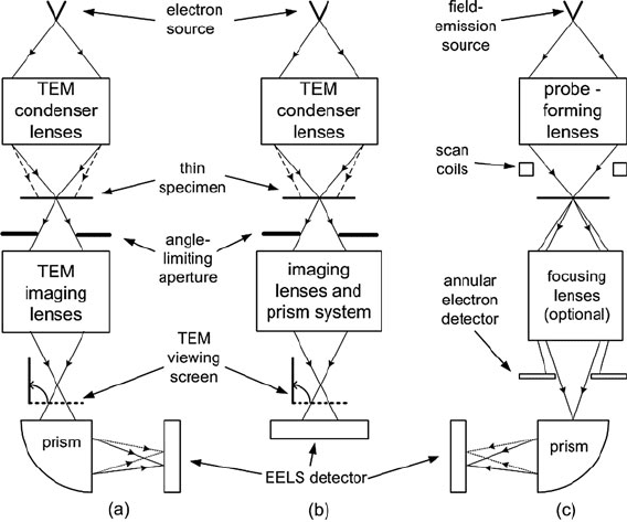
2.6 Energy-Selected Imaging (ESI)
As discussed in Section 2.1, the information carried by inelastic scattering can be
acquired and displayed in several ways, one of these being the energy-loss spec-
trum. In a transmission electron microscope, the volume of material giving rise to
the spectrum can be made very small by concentrating the incident electrons into
a small-diameter probe. EELS can be used to quantitatively analyze this small vol-
ume, the TEM image or diffraction pattern being used to define it relative to its
surroundings (Fig. 2.30a). This process can then be repeated for other regions of
the specimen, either manually or by raster scanning a small probe across the speci-
men and collecting a spectrum from every pixel, as in STEM spectrum imaging; see
Fig. 2.30c. However, it is sometimes useful to display some spectral feature, such as
the ionization edge representing a single chemical element, simultaneously, using
the imaging or diffraction capabilities of a conventional TEM. An image-forming
spectrometer is used as a filter that accepts energy losses within a specified range,
giving an energy-selected image or diffraction pattern. We now discuss several
instrumental arrangements that achieve this capability.
2.6.1 Post-column Energy Filter
As discussed in Section 2.1.1, the magnetic prism behaves somewhat like an electron
lens, producing a chromatically dispersed image of the spectrometer object O at the
plane of an energy-selecting slit or diode array detector. A conventional TEM not
only provides a suitable small-diameter object at its projector lens crossover but also
produces a magnified image or diffraction pattern of the specimen at the level of
2.6 Energy-Selected Imaging (ESI) 99
Fig. 2.30 Three common types of instrument used for EELS and energy-filtered imaging: (a)
imaging filter below the TEM column, (b) in-column filter, and (c) STEM system. In an instrument
dedicated to STEM, the arrangement is often inverted, with the electron source at the bottom
the viewing screen, closer to the spectrometer entrance. The spectrometer therefore
forms a second image, further from its exit, which corresponds to a magnified view
of the specimen or its diffraction pattern. This second image will be energy filtered
if an energy-selecting slit is inserted at the plane of the first image (the energy-loss
spectrum). Slit design is discussed in Section 2.4.4.1.
In general, the energy-filtered image suffers from several defects. Its magnifi-
cation is different in the x- and y-directions, although such rectangular distortion
can easily be corrected electronically if the image is recorded into a computer. It
exhibits axial astigmatism (the spectrometer is double focusing only at the spec-
trum plane), which is correctable by using the dipole-coil stigmators (Shuman and
Somlyo, 1982). More problematic, it may be a chromatic image, blurred in the
x-direction by an amount dependent on the width of the energy-selecting slit. Even
so, by using a 20-μm slit (giving an energy resolution of 5 eV) and a single-prism
spectrometer of conventional design, Shuman and Somlyo (1982) obtained an image
with a spatial resolution of 1.5 nm over a 2-μm field of view at the specimen plane.
The Gatan imaging filter (GIF) uses post-spectrometer multipoles to correct for
these image defects and form a good-quality image or diffraction pattern of the spec-
imen, which is recorded by a CCD camera. Alternatively, the energy-selecting slit
can be withdrawn and the GIF lens system used to project an energy-loss spectrum,
allowing the same camera to be used for spectroscopy, as in Fig. 2.30a. The electron
100 2 Energy-Loss Instrumentation
optics is discussed briefly in Section 2.5.2. Since a modern TEM usually has STEM
capabilities, the GIF can also be used to acquire spectrum images.
2.6.2 In-Column Filters
The prism–mirror and omega filters (Section 2.1.2) were developed specifically
for producing EFTEM images and diffraction patterns. Located in the middle of a
TEM column, they are designed as part of a complete system rather than as add-on
attachments to a microscope. Following the construction of such systems in several
laboratories (Castaing et al., 1967; Henkelman and Ottensmeyer, 1974a,b; Egerton
et al., 1974; Zanchi et al., 1977a; Krahl et al., 1978), energy-selecting microscopes
are now produced commercially (Egle et al., 1984; Bihr et al., 1991; Tsuno et al.,
1997; Koch et al., 2006). Figure 2.31 shows the electron optics of a Zeiss omega-
filter system; the operating modes of this kind of instrument have been described by
Reimer (1991).
Because of the symmetry of these multiple-deflection systems, the image or
diffraction pattern produced is achromatic and has no distortion or axial astig-
matism. Midplane symmetry also precludes second-order aperture aberrations and
image-plane distortion (Rose, 1989). Reduction of axial aberration in the energy-
selecting plane and of field astigmatism and tilt of the final image requires
sextupoles or curved pole faces (Rose and Pejas, 1979; Jiang and Ottensmeyer,
1993), or optimization of the optical parameters (Lanio, 1986; Krahl et al., 1990).
Without such measures, the selected energy loss changes over the field of view,
so that with a narrow energy-selecting slit and no specimen in the microscope, the
zero-loss electrons would occupy a limited area on the final screen, equivalent to
the alignment pattern of a single magnetic prism (Section 2.2.5). Or with an alu-
minum specimen, a low-magnification energy-selected image exhibits concentric
rings corresponding to multiples of the plasmon energy (Zanchi et al., 1977a).
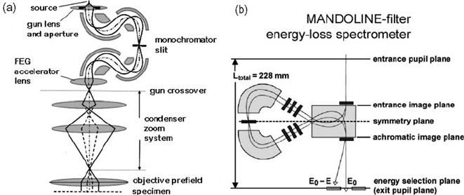
The Zeiss SESAM instrument represents a recent version of this concept (Koch
et al., 2006). It uses a Schottky source, an electrostatic Omega-type filter as a
monochromator and a magnetic MANDOLINE filter as the spectrometer and energy
filter; see Fig. 2.32. To minimize vibrations, the TEM column is suspended at the
level of the objective lens. A comparable project, the JEOL MIRAI instrument, uses
a dual Wien filter as the monochromator and has achieved an energy resolution of
0.14 eV at 200 kV accelerating voltage (Mukai et al., 2004).
2.6.3 Energy Filtering in STEM Mode
Energy filtering is relatively straightforward in the case of a scanning transmission
electron microscope, where the incident electrons are focused into a very small
probe that is scanned over the specimen in a raster pattern. A filtered image can
be viewed simply by directing the output of a single-channel electron detector (as
2.6 Energy-Selected Imaging (ESI) 101
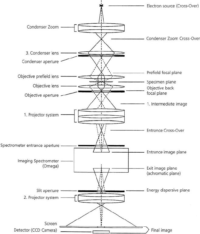
Fig. 2.31 Zeiss EM912 energy-filtering microscope: solid lines show field-defining rays, dashed
lines represent image-defining trajectories. The Omega filter produces a unit-magnification
achromatic image of the specimen (or its diffraction pattern) created by the first group of post-
specimen lenses and generates (at the plane of the energy-selecting slit) a unit-magnification
energy-dispersed image of its entrance crossover. From Carl Zeiss Topics, Issue 4, p. 4
used in serial EELS) to an image display monitor. It is preferable to digitally scan
the probe and to digitize the detector signal so that it can be stored in computer
memory, allowing subsequent image processing.
In STEM mode, the spatial resolution of a filtered image depends on the
incident probe diameter (spot size) and beam broadening in the specimen, but
102 2 Energy-Loss Instrumentation
Fig. 2.32 Components of the Zeiss SESAM instrument: (a) electrostatic omega filter (dispersion
≈ 12 μm/eV at the midplane slit) and (b) MANDOLINE filter, whose dispersion at the energy-
selecting plane exceeds 6 μm/eV
is independent of the spectrometer. For an instrument fitted with a Schottky
or field-emission source, the probe diameter can be below 1 nm or less
than 0.1 nm for an aberration-corrected probe-forming lens (Krivanek et al.,
2008).
If electron lenses are present between the specimen and spectrometer, the mode
of operation of these lenses does affect the energy resolution (Section 2.3.4). Also,
the scanning action of t he probe can result in a corresponding motion of the spec-
trum, due to movement of the spectrometer object point (image coupling) or through
spectrometer aberrations (for diffraction coupling). Different regions of the image
then correspond to different energy loss, limiting the field of view for a given energy
window. The field of view d can be increased by widening the energy-selecting slit,
but this limits the energy resolution to MM
x
d/D (see Section 2.3.5). A preferable
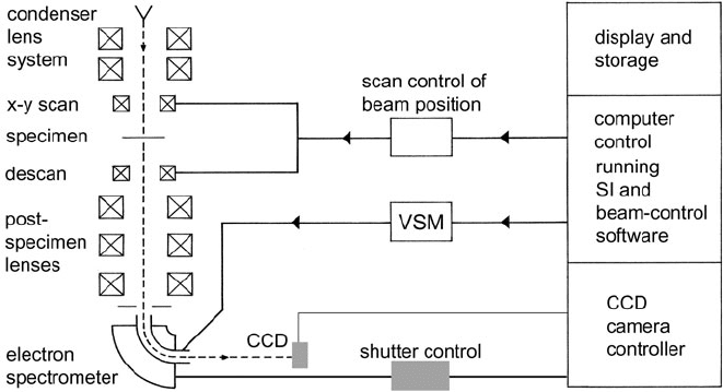
solution is to descan the electron beam by applying the raster signal to dipole scan
coils located after the specimen (Fig. 2.33). Ideally, the field of view is then unlim-
ited and the energy resolution is t he same as for a stationary probe. As there is
no equivalent of descanning in a fixed-beam TEM, the use of STEM mode makes
it easier to obtain good energy resolution i n lower magnification energy-filtered
images.
The STEM spectrometer can also be used to obtain an energy-selected diffraction
pattern, by using x- and y-deflection coils to scan the latter across the spectrome-
ter entrance aperture. However, this method is inefficient, since a large proportion
of the electrons are rejected by the angle-defining aperture. If the required energy
resolution is β and the scan range is ±β, the collection efficiency (and system
DQE) is (β/β)
2
/4. Shorter recording times and lower radiation dose are possible
by using an imaging filter to process the whole diffraction pattern simultaneously
(Krivanek et al., 1994), making the recording of core-loss diffraction patterns more
feasible (Botton, 2005).
2.6 Energy-Selected Imaging (ESI) 103
Fig. 2.33 Scheme for STEM spectrum imaging (Gubbens et al., 2010). A focused probe is scanned
across the specimen and (for lower magnification work) descanned using post-specimen coils. At
each pixel, an extended range of the energy-loss spectrum, chosen by the voltage voltage-scan
module (VSM), is acquired by a parallel-recording spectrometer. An electrostatic shutter within
the spectrometer allows fast switching between the low-loss and core-loss regions of the spectrum
2.6.4 Spectrum Imaging
With a parallel-recording system attached to a scanning-transmission electron
microscope (STEM), the energy-loss spectrum can be read out at each picture point,
creating a four-dimensional data array that corresponds to electron intensity within
a three-dimensional (x, y, E) data cube (Fig. 2.1). The number of intensity values
involved is large: 500 M for a 512 × 512 image, in the case of a 2048-channel spec-
trum. If each spectral intensity is recorded to a depth of 16 bits (64K gray levels), the
total information content is then 0.5 Gbyte if the data are stored as integers (with-
out data compression). However, advances in electronics have made the acquisition
and storage of such data routine (Gubbens et al., 2010). To be efficient, the process
requires good synchronization between the control computer, the CCD camera, and
the probe-scanning and voltage-offset modules; see Fig. 2.33.
An equivalent data set can be obtained from an imaging filter, by reading out
a series of energy-selected images at different energy loss, sometimes called an
image spectrum (Lavergne et al., 1992). Since electrons intercepted by the energy-
selecting slit do not contribute, this process is less efficient than spectrum imaging
and involves a higher electron dose to the specimen, for the same information con-
tent. However, it may involve a shorter recording time, if the incident beam current
divided by the number of energy-selected images exceeds the probe current used
in the s pectrum imaging; see Section 2.6.5. Common problems are undersampling
(dependent on the energy shift between readouts) and a loss of energy resolution
104 2 Energy-Loss Instrumentation
(due to the width of the energy-selecting slit) but these can be addressed by FFT
interpolation and deconvolution methods (Lo et al., 2001).
The main attraction of the spectrum image concept is that more spectroscopic
data are recorded and can be subsequently processed to extract information that
might otherwise have been lost. Examples of such processing include the calculation
of local thickness, pre-edge background subtraction, deconvolution, multivariate
analysis, and Kramers–Kronig analysis. The resulting information can be displayed
as line scans (Tencé et al., 1995) or two-dimensional images of specimen t hickness,
elemental concentration, complex permittivity, and bonding information (Hunt and
Williams, 1991; Botton and L’Esperance, 1994; Arenal et al., 2008). In addition,
instrumental artifacts such as gain nonuniformities and drift of the microscope high
voltage or beam current can be corrected by post-acquisition processing.
The acquisition time of a spectrum image is often quite long. In the past, the min-
imum pixel time has been limited by the array readout time, but that has recently
been reduced from 25 to 1 ms (Gubbens et al., 2010). A line spectrum, achieved by
scanning an electron probe in a line and recording a spectrum from each pixel, can
be acquired more rapidly and is often sufficient for determining elemental profiles.
Similar data can be obtained in fixed-beam TEM mode, with broad beam illumi-
nating a slit introduced at the entrance of a double-focusing spectrometer. The long
direction (y) of the slit corresponds to the nondispersive direction in the spectrome-
ter image plane, allowing the energy-loss intensity J(y,E) to be recorded by a CCD
camera. One advantage here is that all spectra are acquired simultaneously, so spec-
imen drift does not distort the information obtained, although it may result in loss
of spatial resolution.
A common form of energy-filtered image involves selecting a range of energy
loss (typically 10 eV or more in width) corresponding to an inner-shell ioniza-
tion edge. Since each edge is characteristic of a particular element, the core-loss
image contains information about the spatial distribution of elements present in
the specimen. However, each ionization edge is superimposed on a spectral back-
ground arising from other energy-loss processes. To obtain an image that represents
the characteristic loss intensity alone, the background contribution I
b
within the
core-loss region of the spectrum must be subtracted, as in the case of spectroscopy
(Section 4.4). The background intensity often decreases smoothly with energy loss
E, approximating to a power law form J(E) = AE
−r
, where A and r are parameters
that can be determined by examining J(E) at energy losses just below the ionization
threshold (Section 4.4.2). Unfortunately, both A and r can vary across the specimen,
as a result of changes in thickness and composition (Leapman and Swyt, 1983;
Leapman et al., 1984c), in which case a separate estimation of I
b
is required at each
picture element (pixel).
In the case of STEM imaging, where each pixel is measured sequentially, local
values of A and r can be obtained through a least-squares or two-area fitting to the
pre-edge intensity recorded over several channels preceding the edge. With electro-
static deflection of the spectrometer exit beam and fast electronics, the necessary
data processing may be done within each pixel dwell period (“on the fly”) and the
system can provide a live display of the appropriate part of the spectrum (Gorlen
2.6 Energy-Selected Imaging (ESI) 105
et al., 1984), values of A and r being obtained by measuring two or more energy-loss
channels preceding the edge (Jeanguillaume et al., 1978). By recording a complete
line of the picture before changing the spectrometer excitation, the need for fast
beam deflection is avoided, background subtraction and fitting being done off-line
after storing the images (Tencé et al., 1984).
In the case of energy filtering in a fixed-beam TEM, the simplest method of
background subtraction is to record one image at an energy loss just below the ion-
ization edge of interest and subtract some constant fraction of its intensity from
a second image recorded just above the ionization threshold. First done by photo-
graphic recording (Ottensmeyer and Andrew, 1980; Bazett-Jones and Ottensmeyer,
1981), the subtraction process is more accurate and convenient with CCD images.
Nevertheless, this simple procedure assumes that the exponent r that describes the
energy dependence of the background is constant across the image or that the back-
ground is a constant fraction of the core-loss intensity. In practice, r varies as the
local composition or thickness of the specimen changes (Fig. 3.35), making this
two-window method of background subtraction potentially inaccurate (Leapman
et al., 1984c). Variation of r is taken into account in the three-window method by
electronically recording two background-loss images at slightly different energy
loss and determining A and r at each pixel. However, the reduction in systematic
error of background fitting comes at the expense of an increased statistical error
(Section 4.4.3), so a longer recording time is needed for an acceptable signal/noise
ratio (Leapman and Swyt, 1983; Pun and Ellis, 1983).
2.6.4.1 Influence of Diffraction Contrast
Even if the background intensity is correctly subtracted, a core-loss image may be
modulated by diffraction (aperture) contrast, arising from variations in the amount
of elastic scattering intercepted by the angle-limiting aperture. A simple test is
to examine an unfiltered bright-field image, recorded at Gaussian focus using the
same collection aperture; the intensity modulation in this image is a measure of the
amount of diffraction contrast. Several methods have been proposed for removing
this aperture contrast, in order to obtain a true elemental map:
(a) Dividing the core-loss intensity I
k
by a pre-edge background level, to form a
jump-ratio image (Johnson, 1979).
(b) Dividing by the intensity of a low-loss (e.g., first-plasmon) peak, which is also
modulated by diffraction contrast.
(c) Dividing I
k
by the intensity I
l
, measured over an equal energy window in the
low-loss region of the spectrum (Egerton, 1978a; Butler et al., 1982). According
to Eq. (4.65), the ratio I
k
/I
l
is proportional to areal density (number of atoms of
an analyzed element per unit area of the specimen).
(d) Taking a ratio of the core-loss intensities of two elements, giving an image that
represents their elemental ratio; see Eq. (4.66).
(e) Using conical rocking-beam illumination, which varies the angle of incidence
over a wide range (Hofer and Warbichler, 1996).
106 2 Energy-Loss Instrumentation
(f) Recording the filtered images with a large collection semi-angle, so that almost
all the inelastic and elastic scattering enters the spectrometer (Egerton, 1981d;
Muller et al., 2008).
Methods (a), (b), and (d) have the advantage that they correct also for variations
in specimen thickness (if the thickness is not too large), giving an image intensity
that reflects the concentration of the analyzed element (atoms/volume) rather than
its areal density.
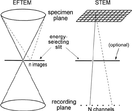
2.6.5 Comparison of Energy-Filtered TEM and STEM
To compare the advantages of the fixed-beam TEM and STEM procedures of energy
filtering, we will assume equal collection efficiency (same β
∗
;seeSection 4.5.3),
similar spectrometer performance in terms of energy resolution over the field of
view, and electron detectors with similar noise properties. We will take the spatial
resolution to be the same in both methods, a resolution below 1 nm being achievable
(for s ome specimens) using either procedure.
Consider first elemental mapping with a TEM imaging filter, in comparison with
a STEM system operating with an energy-selecting slit (as in serial recording). At
any instant, a single energy loss is recorded, energy-selecting slits being present
in both cases; see Fig. 2.34. For two-window background fitting, three complete
images are acquired for each element in either mode, as discussed in the previ-
ous section. For the same amount of information, the electron dose is therefore the
same in both methods. The only difference is that the electron dose is delivered
continuously in the fixed-beam TEM and for a small fraction of the frame time in
STEM mode.
Fig. 2.34 Comparison of
TEM and STEM modes of
energy-selected imaging. The
STEM system can exist with
an energy-selecting slit a nd
single-channel detector (serial
recording spectrometer) or
without the slit, allowing the
use of parallel recording
(spectrum image mode)
2.6 Energy-Selected Imaging (ESI) 107
In the STEM case, the dose rate (current density in the probe) can be consider-
ably higher than for broad-beam TEM illumination. Whether an equal dose implies
the same amount of radiation damage to the specimen then depends on whether the
radiation damage is dose rate dependent. For polymer specimens, temperature rise
in the beam can increase the amount of structural damage for a given dose (Payne
and Beamson, 1993). In some inorganic oxides, mass loss (hole drilling) occurs
only at the high current densities such as are possible in a field-emission STEM (see
Section 5.7.5). For such specimens, the STEM procedure would be more damaging,
for the same recorded information.
The recording time for a single-element map is generally longer in STEM, since
the probe current (even with a field-emission source) is typically below 1 nA,
whereas the beam current in a conventional TEM can be as high as 1 μA. STEM
recording of a 512 × 512-pixel image may take as much as 1 h to achieve adequate
statistics, which is inconvenient and requires specimen drift correction. The usual
solution is to reduce the amount of information recorded by decreasing the number
of pixels. In a conventional TEM, the CCD camera offers typically 2k × 2k pixels,
so EFTEM can provide a higher information rate.
When a parallel-recording spectrometer is used in the STEM, the three images
required for each element are recorded simultaneously, reducing both the time and
the dose by a factor of 3. This factor becomes 3n in a case where n ionization edges
are recorded simultaneously. STEM with a parallel-recording spectrometer should
therefore produce less radiation damage than an energy-filtering TEM, unless dose
rate effects occur that outweigh this advantage.
The advantage of STEM is increased further when an extended range of energy
loss is recorded by the diode array, as in spectrum imaging. If use is made of the
information recorded by all N detector channels, a given electron dose to the spec-
imen yields N times as much information as in EFTEM, where N energy-selected
images would need to be acquired sequentially to form an image spectrum of equal
information content. STEM spectrum imaging also makes it easier to perform on-
or off-line correction for specimen drift, so that long recording times (although
inconvenient) do not necessarily compromise the spatial resolution of analysis. The
acquisition time in STEM could actually be shorter if the product NI
p
, where I
p
is
the probe current, exceeds the beam current used for EFTEM imaging.
Both scanning and fixed-beam modes of operation are possible in a conventional
TEM equipped with probe scanning and (preferably) a field-emission source and
parallel-recording spectrometer. With such an instrument, single-element imaging
is likely to be faster in EFTEM mode, but in the case of multielement imaging or
the need for data covering a large range of energy loss, the STEM mode is more
efficient in terms of specimen dose and (possibly) acquisition time.
The above arguments assume that the whole of the imaged area is uniformly irra-
diated in STEM mode, just as it is in EFTEM. However, if the STEM probe size
were kept constant and the magnification reduced, only a fraction of the pixel size
would be irradiated by the probe; radiation damage would be higher than necessary,
with regions between scan lines or probe positions (for a digital scan) left unirra-
diated. In other words, the specimen would be undersampled by the probe. One