Durst F. Fluid Mechanics: An Introduction to the Theory of Fluid Flows
Подождите немного. Документ загружается.

614 19 Numerical Solutions of the Basic Equations
When subsequently a
α
P
=ˇa
α
P
−S
α
P
∗
∆V and b = S
α
c
∆V +
ρ∆V
∆t
Φ
α−1
P
is set,
the completely discretized form of (19.32) results:
a
α
P
Φ
α
P
−
Nb
a
α
Nb
Φ
α
Nb
= b. (19.99)
19.5 Computation of Laminar Flows
When one analyzes the general Navier–Stokes equations and the energy equa-
tion for an incompressible fluid, i.e. the general transport equation, it can be
demonstrated that we have a set of partial differential equations which shows
a parabolic time response and an elliptic space behavior. Because of this time
response and space behavior, initial conditions at the point of time t =0have
to be given, and the boundary conditions have to be specified along the en-
tire area of the borders of the flow area. It is usual to include the following
boundary conditions into the numerical computations:
• The Dirichlet boundary conditions: Descriptions of the values of all
variables along the boundaries of the computational area
• The Neumann boundary conditions: Descriptions of the gradients (or of the
diffusive fluxes) of the variables along the boundaries of the computational
area
• A combination of the Dirichlet and Neumann boundary conditions
• Periodic boundary conditions
Thus, for practical computations, specific boundary conditions result for:
– Solid walls
– Symmetry planes
– Inflow planes
– Outflow planes
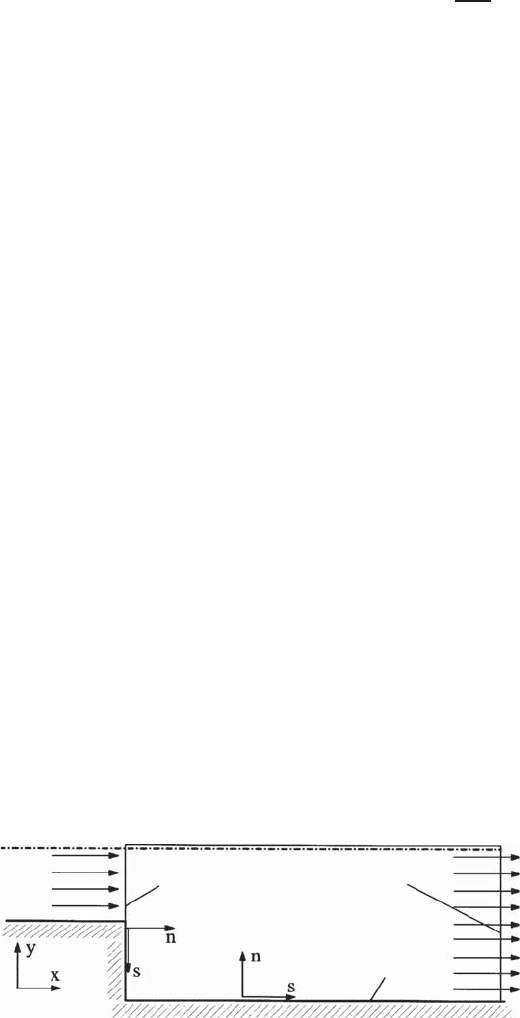
which can be considered separately; for this purpose, the s − n coordinate
system of Fig. 19.11 is used.
Plane of symmetry
Inlet plane
Outlet plane
Solid wall
Fig. 19.11 Diagram explaining possible boundary conditions

19.5 Computation of Laminar Flows 615
19.5.1 Wall Boundary Conditions
On walls the no-slip boundary condition is employed. For impermeable
surfaces, both velocities are set at zero, i.e.
U
s
= U
n
=0. (19.100)
For the temperature either the wall temperature or the wall heat flux values
can be specified:
T = T
w
or
∂T
∂n
= −
Pr
µc
p
Q
w
, (19.101)
where T
w
designates the wall temperature and Q
w
the wall heat flux per unit
area (heat flux density).
19.5.2 Symmetry Planes
At symmetry planes, the normal gradients (or fluxes) of the tangential veloc-
ity and all scalar variables are zero. In addition, the velocity normal to the
symmetry plane disappears:
∂U
s
∂n
= U
n
=
∂T
∂n
=0. (19.102)
19.5.3 Inflow Planes
At inflow planes the profiles of U
s
,U
n
and T are normally prescribed by
tabulated data or by analytical functions.
19.5.4 Outflow Planes
If the outflow planes are of the type where the flow shows parabolic behavior
and the plane is sufficiently far away from the flow region of interest, a fully
developed flow can be assumed, i.e. the gradients in the flow direction can be
neglected:
∂U
s
∂n
=
∂U
n
∂n
=
∂T
∂n
=0. (19.103)
The specification of profiles for U
s
, U
n
and T is also possible.
With boundary conditions of this kind, laminar flows as represented in
Figs. 19.12–19.14 can now be computed.
616 19 Numerical Solutions of the Basic Equations
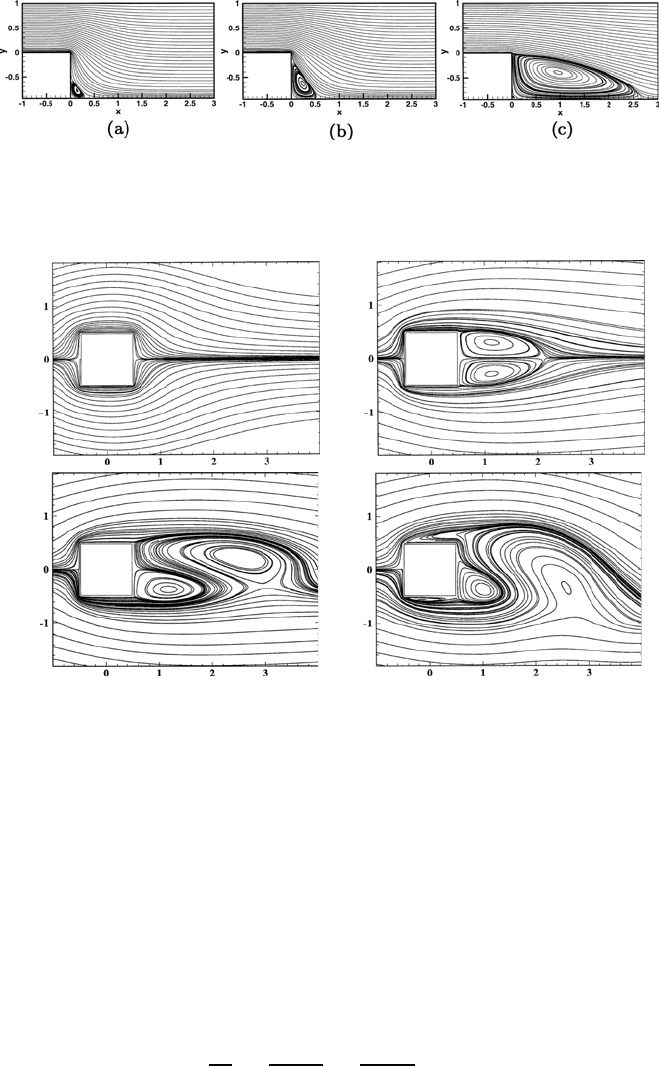
Fig. 19.12 Computations of flows with different Reynolds numbers in a two-
dimensional flow channel with a backward facing step; Re =10
−4
(a), Re =10
(b), Re = 100 (c)
a)
b)
c) d)
Fig. 19.13 Computations of flows for the flow around a two-dimensional cylinder
with square cross-sectional area; Re =1(a), Re =30(b), Re =60(c), Re = 200 (d)
19.6 Computations of Turbulent Flows
19.6.1 Flow Equations to be Solved
Computations of turbulent flows, in the presence of high Reynolds numbers,
require the solution of the Reynolds transport equations that were derived
in Chap. 17 and for which, for two-dimensional flows, areas can be stated as
follows:
Mass Conservation (Continuity Equation):
∂ρ
∂t
+
∂(ρU)
∂x
+
∂(ρV )
∂y
=0. (19.104)
19.6 Computations of Turbulent Flows 617
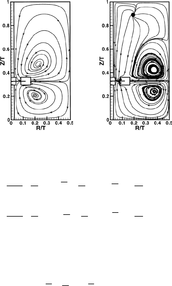
(a) (b)
Fig. 19.14 Results of laminar flow computations in a stirred vessel with inserted
Rushton turbine; (a) Re =1,(b) Re = 100; Breuer (2002)
Momentum Conservation in the x-Direction:
∂(ρU)
∂t
+
∂
∂x
(ρU
2
+ ρu
2
)+
∂
∂y
(ρUV + ρ
uv)=−
∂P
∂x
. (19.105)
Momentum Conservation in the y-Direction:
∂(ρV )
∂t
+
∂
∂x
(ρUV + ρ
uv)+
∂
∂y
(ρV
2
+ ρv
2
)=−
∂P
∂y
. (19.106)
For turbulent flows, all variables designated by capital letters and the thermo-
dynamic fluid properties have to be interpreted as time-averaged quantities.
Fluctuating flow quantities are designated by lower-case letters. Mean values
of turbulent velocity fluctuation, resulting in correlations of the fluctuations,
are indicated by overbars. The molecule-dependent momentum transports in
the momentum equations are neglected in the following, which is justified by
the assumption that high Reynolds numbers are involved. This assumption
is a customary approximation, when computing elliptical turbulent flows.
The correlations −ρ
u
2
, −ρuv and −ρv
2
represent the momentum transport
by the turbulent fluctuating velocity components. They act like “stresses” on
the considered fluid elements and are therefore defined as Reynolds stresses.
These stresses are additional unknowns in the equation system (19.104)–
(19.106) and have to be related via a turbulence model to “known quantities.”
618 19 Numerical Solutions of the Basic Equations
To make a complete solution of the flow equations possible, the set of
equations needs to be closed.
The k− turbulence model (Launder and Spalding, 1972) makes use of the
eddy-viscosity hypothesis, which relates the Reynolds stresses to the mean
flow deformation rates in the following way:
−ρ
u
2
=2µ
t
∂U
∂x
−
2
3
ρk, (19.107)
−ρ
v
2
=2µ
t
∂V
∂y
−
2
3
ρk, (19.108)
−ρ
uv = µ
t
∂U
∂y
+
∂V
∂x
. (19.109)
The proportionality factor µ
t
is the eddy viscosity. The quantity k, appearing
in (19.107) and (19.108), is the turbulent kinetic energy, which is equal to
half the sum of the normal Reynolds stresses (divided by the density):
k =
1
2
u
2
+ v
2
+ w
2
(19.110)
and w is the fluctuation of the velocity in the z direction. The eddy viscosity
µ
t
is not a fluid property, but depends on the local turbulent flow conditions.
When one writes the above x–y momentum equations in the form which
corresponds to the general transport equation, one obtains:
∂(ρU)
∂t
+
∂
∂x
ρU
2
− µ
t
∂U
∂x
+
∂
∂y
ρUV − µ
t
∂U
∂y
= −
∂P
∗
∂x
+ S
U
,
∂(ρV )
∂t
+
∂
∂x
ρUV − µ
t
∂V
∂x
+
∂
∂y
ρV
2
− µ
t
∂V
∂y
= −
∂P
∗
∂y
+ S
V
(19.111)
with the source terms:
S
U
=
∂
∂x
µ
t
∂U
∂x
+
∂
∂y
µ
t
∂V
∂x
, (19.112)
S
V
=
∂
∂x
µ
t
∂U
∂y
+
∂
∂y
µ
t
∂V
∂y
. (19.113)
The modified pressure term P
∗
is equal to:
P
∗
= P +
2
3
ρk. (19.114)
In most cases relevant in practice we have P
2
3
ρk,sothatP = P
∗
can be
set without introducing a serious error.
19.6 Computations of Turbulent Flows 619
The conservation of the time-averaged or ensemble-averaged energy results
in a transport equation for the temperature described by
∂(ρc
p
T )
∂t
+
∂
∂x
!
ρc
p
UT + ρc
p
ut
"
+
∂
∂y
!
ρc
p
VT + ρc
p
vt
"
= S
T
, (19.115)
where t is the fluctuating value of T ,and−ρc
p
ut and −ρc
p
vt represent turbu-
lent energy-flux values. The terms for the molecular transport were already
neglected in (19.115). For Prandtl numbers around 1, this agrees with the
assumption that was made when deriving the conservation equation for the
momentum of turbulent flows.
For turbulent flows, the turbulent energy transport terms are related to
the mean temperature gradients by an eddy diffusivity concept:
−ρc
p
ut =
µ
t
c
p
Pr
t
∂T
∂x
, (19.116)
−ρc
p
vt =
µ
t
c
p
Pr
t
∂T
∂y
. (19.117)
The eddy viscosity µ
t
is employed in the expression from the k − turbulence
model. The turbulent Prandtl number Pr
t
is an empirical constant which is
specified in the next section. The introduction of (19.116) into (19.115) yields
the temperature equation to be solved for turbulent flow predictions:
∂(ρc
p
T )
∂t
+
∂
∂x
ρc
p
UT −
µ
t
c
p
Pr
t
∂T
∂x
+
∂
∂y
ρc
p
VT −
µ
t
c
p
Pr
t
∂T
∂y
= S
T
.
(19.118)
The definition of µ
t
, in many practical cases, takes place through the k −
turbulence model, where dimensional considerations lead to the following
relationship concerning the eddy viscosity:
µ
t
= ρc
µ
k
2
/,
k = turbulent kinetic energy,
= turbulent rate of dissipation,
(19.119)
where c
µ
is an empirical constant which is given below. Local values of k and
are obtained by solving the semi-empirical transport equations for k and ,
which read as follows:
∂(ρk)
∂t
+
∂
∂x
ρUk −
µ
t
σ
k
∂k
∂x
+
∂
∂y
ρV k −
µ
t
σ
k
∂k
∂y
= P
k
− ρ, (19.120)
∂(ρ)
∂t
+
∂
∂x
ρU −
µ
t
σ
∂
∂x
+
∂
∂y
ρV −
µ
t
σ
∂
∂y
=
k
(c
1
P
k
− c
2
ρ). (19.121)
620 19 Numerical Solutions of the Basic Equations
The terms on the left-hand sides of these equations represent the changes
of k and with time and their “transport” through the time-averaged and
fluctuating turbulent motions in the flow. The right-hand sides contain the
production and “destruction” rates. In the k equation, the “k destruction
rate” is set equal to the dissipation rate multiplied by the density. The
production rate P
k
is defined as
P
k
= µ
t
2
∂U
∂x
2
+2
∂V
∂y
2
+
∂U
∂y
+
∂V
∂x
2
5
. (19.122)
For the empirical constants c
1
, c
2
, σ
k
, σ
and c
µ
, usually the standard
values suggested by Launder and Spalding (1974) are assumed. For flows
limited by walls and for free flows, values of 0.6 and 0.86 are recommended
for the turbulent Prandtl number. The k − model constants are summarized
in Table 19.2.
The transport equations presented above for turbulent flows can be
written, in a general form, as follows:
∂(ρΦ)
∂t
+
∂∂
∂∂x
ρUΦ − Γ
Φ
∂Φ
∂x
+
∂
∂y
ρV Φ − Γ
Φ
∂Φ
∂y
= S
Φ
, (19.123)
where Φ represents U , V , T , k or . The diffusion coefficients Γ
Φ
and the
source terms S
Φ
for turbulent flows are compiled in Table 19.3. For laminar
flows, the eddy viscosity and the turbulent Prandtl number are replaced by
corresponding molecular values and the k and transport equations do not
have to be solved.
19.6.2 Boundary Conditions for Turbulent Flows
19.6.2.1 Wall Boundary Conditions
For specifying the wall boundary conditions, usually the wall function method
(Launder and Spalding, 1972) is used, which bridges the viscous wall-near
Table 19.2 Empirical constants of the k − turbulence models
c
µ
c
1
c
2
σ
k
σ
Pr
t
0.09 1.44 1.92 1.0 1.3 0.6–0.86
Table 19.3 Diffusivity and source terms for general transport equation (19.123)
ΦΓ
Φ
S
Φ
Uµ
t
−∂P/∂x + ∂/∂x(µ
t
∂U/∂x)+∂/∂y(µ
t
∂V/∂x)
Vµ
t
−∂P/∂y + ∂/∂x(µ
t
∂U/∂y)+∂/∂y(µ
t
∂V/∂y)
Tµ
t
c
p
/P r
t
S
T
kµ
t
/σ
k
P
k
− ρ
µ
t
/σ
/k(c
1
P
k
− ρc
2
)
19.6 Computations of Turbulent Flows 621
regions with empirical assumptions. Using wall functions in the near-wall
region, instead of resolving the viscous sublayers, offers two advantages:
• The computational time and the required computer storage of data are
both reduced because the high gradients of all the dependent variables
near the wall need not be resolved.
• Some of the assumptions made in the derivation of the k − models lose
their validity in the viscosity-dominant near-wall zone, hence this fact does
not need to be considered.
For the wall functional method, the first grid node away from the wall, for
the numerical computations, has to be localized in the fully turbulent area,
according to the diagram in Fig. 19.15. Typical dimensionless wall distances
which characterize this region are stated below.
In the case of the wall-parallel velocity, the wall functional method suggests
an equation which relates the wall shear stress τ
w
(i.e. the momentum flow
through the control volume close to the wall) to the velocity at the first grid
node U
s,c
away from the wall and to the distance n
c
of this point to the wall.
The basis for this equation is the logarithmic velocity law:
U
s,c
τ
w
/ρ
=
1
κ
ln
n
c
√
ρτ
w
µ
+ C =
1
κ
ln
E
n
c
√
ρτ
w
µ
. (19.124)
Values for the von Karman constant κ and the roughness parameter C
are given in Table 19.4. It should be noted that the value given for C in
Table 19.4, holds for hydrodynamically smooth surfaces only. For rough walls,
other values of C are needed.
Grid points
Control volume
Wall
Fully turbulent
region
Viscous sublayer
Fig. 19.15 Control volume near the wall
Table 19.4 Constants in the logarithmic wall law
κCE= e
κC
0.41 5.2 8.43171
622 19 Numerical Solutions of the Basic Equations
Equation (19.124) is transcendental in τ
w
and becomes singular at sepa-
ration points (where τ
w
→0). Because of these problems, a modified form
of (19.124) is often used. The extension is built on the following three
assumptions for the flow in the near-wall control volumes:
• Directly near the wall, a Couette flow exists, with δ/δs =0,andU
n
=0
• The production and dissipation rates are in equilibrium, i.e. local
equilibrium of the turbulence
• There is a layer of constant stress, with −ρ
u
s
u
n
= τ
w
The logarithmic law for the mean velocity and the above three assumptions
does not hold in the proximity of or within separation areas.
When assuming a Couette flow, the eddy-viscosity relationship (19.109)
becomes
−ρ
u
s
u
n
= µ
t
∂U
s
∂n
= ρc
µ
k
2
∂U
s
∂n
(19.125)
and the local equilibrium condition (production rate = dissipation rate) is
expressed as follows:
−ρ
u
s
u
n
∂U
s
∂n
= ρ. (19.126)
On inserting (19.126) into (19.125), the following results:
k =
−
u
s
u
n
√
c
µ
(19.127)
and the assumption of a layer of constant stress leads to
τ
w
/ρ =
√
c
µ
k. (19.128)
From (19.128) and the logarithmic velocity law (19.124), one obtains, by
simple algebraic derivations, an explicit relationship for the wall shear stress:
τ
w
=
ρκc
1/4
µ
k
1/2
c
ln(En
∗
c
)
U
s,c
(19.129)
with the dimensionless wall distance
n
∗
c
=
ρc
1/4
µ
k
1/2
c
n
c
µ
. (19.130)
Equations (19.129) and (19.130) are used in most computer programs. These
equations hold in the range
30 <n
∗
c
< 500. (19.131)
One should therefore place the grid nodes of the wall-nearest control volumes
carefully in this range.
19.6 Computations of Turbulent Flows 623
19.6.2.2 Standard Velocity
As in the case of laminar flows, the standard velocity at the wall, and also
its gradient, are equal to zero. The wall function takes care of the difference
from the correct velocity gradient.
19.6.2.3 Temperature
The near-wall distribution for the temperature is based on similarity argu-
ments for the inner wall layer, from which (for low Mach numbers) a linear
relationship results between the temperature and the velocity. The often used
temperature law reads
(T
c
− T
w
)ρc
p
c
1/4
µ
k
1/2
c
Q
w
=
Pr
t
κ
ln n
∗
c
+ C
Q
(Pr). (19.132)
The additive constant C
Q
is a function of the molecular Prandtl number Pr.
To determine it, an empirical relationship is employed:
C
Q
=12.5Pr
2/3
+2.12 lnPr− 5.3forPr > 0.5, (19.133)
C
Q
=12.5Pr
2/3
+2.12 ln Pr− 1.5forPr ≤ 0.5. (19.134)
Equation (19.132) can easily be resolved according to the wall heat flux
Q
w
, which is the quantity of interest for the implementation of the wall
temperature into the finite-volume methods computational procedure.
19.6.2.4 Turbulent Kinetic Energy
Immediately near the wall, the turbulent kinetic energy k changes quadrati-
cally with the wall distance, i.e. k ∝ n
2
c
. At the same time, the diffusive wall
flow of k has the value zero:
µ
t
σ
k
∂k
∂n
=0. (19.135)
In addition to the application of (19.135), the production and dissipation rates
in the wall-nearest control volumes are determined approximately, logically
assuming a Couette flow, a local equilibrium and a constant stress layer, as
discussed previously. This is described in the following. With (19.122), the
production rate of the kinetic energy in the wall-nearest control volumes is
computed with
P
k
=
τ
2
w
ρκc
1/4
µ
k
1/2
c
n
c
, (19.136)