Durst F. Fluid Mechanics: An Introduction to the Theory of Fluid Flows
Подождите немного. Документ загружается.

604 19 Numerical Solutions of the Basic Equations
methods only values of Φ at the grid points are stored, as only they are
of interest for the solution and later computations. As a consequence, the
values Φ
cf
have to be expressed as functions of the values Φ
Nb
of the grid
points neighboring the considered control volume surface. Computing the
values Φ
cf
from Φ
Nb
, required for the computational methods, is the actual
difficulty when discretizing the basic fluid mechanics equations by means of
finite-volume methods. There is the problem, as already stated above, when
applying the mean integral value theorem, that the behavior of Φ as a func-
tion of space should be known between two grid points, in order to be able to
derive the exact values of Φ
cf
or
∂Φ
∂x
|
cf
at each of the considered control vol-
ume surfaces. However, it is exactly this behavior which has to be computed,
and it is therefore necessary for the derivations of the computational scheme
to assume a behavior. This assumption represents the third approximation
step of the finite-volume method considered here.
A certain understanding of the introduced approximation can be found
by considering a simplified problem. The equation for a one-dimensional,
stationary flow problem, without sources, is
d
dx
ρuΦ − Γ
dΦ
dx
=0. (19.50)
For this equation, an analytical solution can be found:
Φ ∼ exp
(ρu)x
Γ
. (19.51)
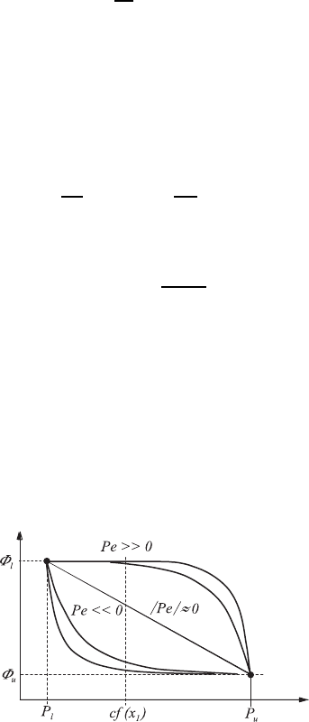
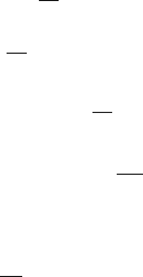
In Fig. 19.9, the behavior of this solution of the above equation is represented
for a boundary value problem between two points P
l
and P
u
with the cor-
responding functional values Φ
l
and Φ
u
. The functional relationship is given
as a function of the Peclet number. The Peclet number represents the ratio
between the convective and diffuse transport of Φ.
On considering Fig. 19.9 and also the solution of the transport equation
(19.50), it is actually obvious to assume an exponential behavior of Φ between
the grid points also in the multi-dimensional flow case. However, the compu-
tation of exponential functions on a computer is very costly compared with
Fig. 19.9 Dependence of the behavior of Φ on the mass current density (Peclet
number)
19.4 Finite-Volume Discretization 605
other operations, and one is inclined to approximate the actual functional
behavior by a polynomial. The various approximation ansatzes employed for
this differs in the order of the polynomial used. In the present section, those
polynomials of zero and first order will be considered, which lead to the
so-called Upwind or central differential methods.
Owing to the assumption of a linear distribution of Φ between the two grid
points, the derivation for the diffusive transport term can approximately be
replaced by:
∂Φ
∂x
cf
=
Φ
u
− Φ
l
δx
cf
. (19.52)
The flow through the control-volume surface cf can then be approximated
as follows:
−Γ
∗
cf
∂Φ
∂x
cf
∆A
cf
=
Γ
∗
cf
∆A
cf
δx
cf
(Φ
l
− Φ
u
)=D
∗
cf
(Φ
l
− Φ
u
) (19.53)
and one obtains for the different control-volume sides:
cf = w, s, b : −Γ
∗
cf
∂Φ
∂x
cf
∆A
cf
= D
∗
cf
(Φ
Nb
− Φ
P
), (19.54)
cf = e, n, t : −Γ
∗
cf
∂Φ
∂x
cf
∆A
cf
= D
∗
cf
(Φ
P
− Φ
Nb
), (19.55)
where Nb is the neighboring point of cf with the direction being given by P
and the location of the considered surface.
For the approximation of the convective fluxes, differing approximate con-
siderations can now be used, yielding different computational methods; they
are explained below.
19.4.2.1 Upwind Method
The upwind method approximates the behavior of Φ between two grid points
by a polynomial of zero order, i.e. a constant. From Fig. 19.9, one recognizes
quickly that this approximation is good for large Peclet numbers, i.e. for
situations in which the convective transport is predominant. For this case,
the value of Φ at the P -surface differs only slightly from the value at the
grid point located upwind of cf . It is thus also clear by which value of Φ the
approximation should be introduced, i.e. always by the one located upwind
of cf. For a flow in the positive coordinate direction, this is Φ
l
, and for the
negative direction, it is Φ
u
. It is therefore necessary to be able to determine
the flow direction at the control-volume surfaces. For this purpose, we shall
use the mass flux:
m
∗
cf
=(ρu)
∗
cf
∆A
cf
. (19.56)
606 19 Numerical Solutions of the Basic Equations
For each control-volume surface, the direction of the mass flux has to be
determined by means of its plus/minus sign. Therefore, the following needs
to be considered:
cf = w, s, b : Φ
cf
=
Φ
Nb
for m
∗
cf
> 0
Φ
P
for m
∗
cf
< 0,
(19.57)
cf = e, n, t : Φ
cf
=
Φ
P
for m
∗
cf
> 0
Φ
Nb
for m
∗
cf
< 0.
(19.58)
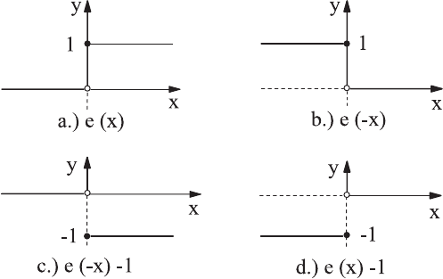
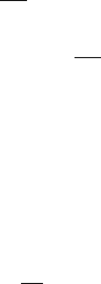
To be able to represent all possible combinations of the above expressions
by a uniform notation, we introduce a unit “step function,” which is defined
as follows:
e(x)=
1forx ≥ 0
0forx<0.
(19.59)
This function is sketched in Fig. 19.10. The function for which the step is
carried out for negative x is given as follows:
e(−x)=
0forx>0
1forx ≤ 0
(19.60)
and it is represented by Fig. 19.10b. With this, the functions e(x) given in
(19.57) can be written as:
cf = w, s, b : Φ
cf
= e
!
m
∗
cf
"
Φ
Nb
+ e
!
−m
∗
cf
"
Φ
P
, (19.61)
cf = e, n, t : Φ
cf
= e
!
−m
∗
cf
"
Φ
Nb
+ e
!
m
∗
cf
"
Φ
P
. (19.62)
On inserting these expressions for the convective and also the diffusive terms
into (19.47), one obtains:
Fig. 19.10 Unit step function

19.4 Finite-Volume Discretization 607
∂
∂t
(ρ
∗
P
Φ
P
)∆V +(m
∗
e
(e(−m
∗
e
)Φ
E
+ e(m
∗
e
)Φ
P
)+D
∗
e
(Φ
P
− Φ
E
)) −
(m
∗
w
(e(m
∗
w
)Φ
W
+ e(−m
∗
w
)Φ
P
)+D
∗
w
(Φ
W
− Φ
P
)) +
(m
∗
n
(e(−m
∗
n
)Φ
N
+ e(m
∗
n
)Φ
P
)+D
∗
n
(Φ
P
− Φ
N
)) −
(m
∗
s
(e(m
∗
s
)Φ
S
+ e(−m
∗
s
)Φ
P
)+D
∗
s
(Φ
S
− Φ
P
)) +
(m
∗
t
(e(−m
∗
t
)Φ
T
+ e(m
∗
t
)Φ
P
)+D
∗
t
(Φ
P
− Φ
T
)) −
(m
∗
b
(e(m
∗
b
)Φ
B
+ e(−m
∗
b
)Φ
P
)+D
∗
b
(Φ
B
− Φ
P
)) = S
P
∆V
(19.63)
and with a little rearrangement of the terms of this equation, the total
expression then reads:
ρ
∗
P
∂Φ
P
∂t
∆V +(m
∗
e
(e(−m
∗
e
)Φ
E
+(e(m
∗
e
) − 1)Φ
P
)+D
∗
e
(Φ
P
− Φ
E
)) −
(m
∗
w
(e(m
∗
w
)Φ
W
+(e(−m
∗
w
) − 1)Φ
P
) − D
∗
w
(Φ
P
− Φ
W
)) +
(m
∗
n
(e(−m
∗
n
)Φ
N
+(e(m
∗
n
) − 1)Φ
P
)+D
∗
n
(Φ
P
− Φ
N
)) −
(m
∗
s
(e(m
∗
s
)Φ
S
+(e(−m
∗
s
) − 1)Φ
P
) − D
∗
s
(Φ
P
− Φ
S
)) +
(m
∗
t
(e(−m
∗
t
)Φ
T
+(e(m
∗
t
) − 1)Φ
P
)+D
∗
t
(Φ
P
− Φ
T
)) −
(m
∗
b
(e(m
∗
b
)Φ
B
+(e(−m
∗
b
) − 1)Φ
P
) − D
∗
b
(Φ
P
− Φ
B
)) +
!
∂ρ
∗
P
∂t
∆V + m
∗
e
− m
∗
w
+ m
∗
n
− m
∗
s
+ m
∗
t
− m
∗
b
=0
"
Φ
P
= S
P
∆V.
(19.64)
As indicated before, the term covered by the brace represents the continu-
ity equation in its discrete form and therefore disappears because of (19.49).
A necessary requirement for this is that the iteration process secures the mass
conservation after each iteration step.
The above equation contains the expressions e(−m
∗
cf
) −1ande(m
∗
cf
) −1.
These functions are also represented in Fig. 19.10. One realizes from their
behavior that the following holds:
e(x) − 1=−e(− x)ande(−x) − 1=−e(x). (19.65)
On considering this e(x)ande(−x) behavior, equation (19.64) can be
simplified further:
ρ
∗
P
∂Φ
P
∂t
∆V +
(−m
∗
e
e(−m
∗
e
)+D
∗
e
)(Φ
P
− Φ
E
) − (−m
∗
w
e(m
∗
w
) − D
∗
w
)(Φ
P
− Φ
W
)+
(−m
∗
n
e(−m
∗
n
)+D
∗
n
)(Φ
P
− Φ
N
) − (−m
∗
s
e(m
∗
s
) − D
∗
s
)(Φ
P
− Φ
S
)+
(−m
∗
t
e(−m
∗
t
)+D
∗
t
)(Φ
P
− Φ
T
) − (−m
∗
b
e(m
∗
b
) − D
∗
b
)(Φ
P
− Φ
B
)=S
P
∆V
(19.66)

608 19 Numerical Solutions of the Basic Equations
and one can introduce the abbreviation a
Nb
for the coefficients of the terms
(Φ
P
− Φ
Nb
):
Nb = W, S, B : a
Nb
= D
∗
cf
+ m
∗
cf
e(m
∗
cf
),
Nb = E,N,T : a
Nb
= D
∗
cf
− m
∗
cf
e(−m
∗
cf
).
(19.67)
The expressions, which now also contain the unit step function, can
also be expressed by means of the function max[a, b], which exists in most
programming languages and which expresses the larger of the two values:
Nb = W, S, B : a
Nb
= D
∗
cf
+max[m
∗
cf
, 0],
Nb = E,N,T : a
Nb
= D
∗
cf
+max[0, −m
∗
cf
].
(19.68)
When using the coefficients a
Nb
, one obtains from (19.65):
ρ
∗
P
∂Φ
P
∂t
∆V + a
E
(Φ
P
− Φ
E
)+a
W
(Φ
P
− Φ
W
)+
a
N
(Φ
P
− Φ
N
)+a
S
(Φ
P
− Φ
S
)+
a
T
(Φ
P
− Φ
T
)+a
B
(Φ
P
− Φ
B
)=S
P
∆V.
(19.69)
After inserting the following abbreviation:
ˆa
P
= a
E
+ a
W
+ a
N
+ a
S
+ a
T
+ a
B
=
Nb
a
Nb
(19.70)
one finally obtains:
ρ
∗
P
∂Φ
P
∂t
∆V +ˆa
P
Φ
P
−
Nb
a
Nb
Φ
Nb
= S
P
∆V. (19.71)
This equation is the discrete analogue of (19.32) after discretization of
the differentials with respect to space by means of the upwind method. The
coefficients can be computed according to (19.68).
19.4.2.2 Central Difference Method
The central difference method approximates the exponential behavior of Φ,
between two grid points, by a polynomial of first order. This corresponds to
the assumption of a linear variation of Φ, which represents a good approxi-
mation for small Peclet numbers. The behavior of Φ is approximated all the
better by this method, the more the diffusive transport prevails in the flow
and the more diffusive transports of properties are present.
19.4 Finite-Volume Discretization 609
A linear behavior of Φ between two grid points P
l
and P
u
can
be expressed by
Φ(x)=Φ
l
+
Φ
u
− Φ
l
δx
cf
[x − 1/2(x
l
+ x
ll
)] for x
l
≤ x ≤ x
u
. (19.72)
On representing δx
cf
by the stored coordinates at the grid points, the
following results:
δx
cf
=1/2(x
u
− x
ll
). (19.73)
The control surface is just located at point x = x
l
, so that one can write
Φ
cf
= Φ
l
+
Φ
u
− Φ
l
1/2(x
u
− x
ll
)
(x
l
− 1/2x
l
− 1/2x
ll
)
= Φ
l
+(Φ
u
− Φ
l
)
(x
l
− x
ll
)
(x
u
− x
ll
)
.
(19.74)
By the definition of the interpolation coefficient as
η
cf
=
x
l
− x
ll
x
u
− x
ll
(19.75)
an equation can be derived for the interpolation of the control surface values,
employing the values of the neighboring grid points:
Φ
cf
= η
cf
Φ
u
+(1− η
cf
)Φ
l
. (19.76)
For all occurring control-volume sides, one thus obtains
cf = w, s, b : Φ
cf
= η
cf
Φ
P
+(1− η
cf
)Φ
Nb
, (19.77)
cf = e, n, t : Φ
cf
= η
cf
Φ
Nb
+(1− η
cf
)Φ
P
. (19.78)
On inserting these expressions and again the approximations for the diffusive
flows (19.54) and (19.47) in (19.47), one obtains
∂
∂t
(ρ
∗
P
Φ
P
)∆V +(m
∗
e
(η
e
Φ
E
+(1− η
e
)Φ
P
)+D
∗
e
(Φ
P
− Φ
E
)) −
(m
∗
w
(η
w
Φ
P
+(1− η
w
)Φ
W
)+D
∗
w
(Φ
W
− Φ
P
)) +
(m
∗
n
(η
n
Φ
N
+(1− η
n
)Φ
P
)+D
∗
n
(Φ
P
− Φ
N
)) −
(m
∗
s
(η
s
Φ
P
+(1− η
s
)Φ
S
)+D
∗
s
(Φ
S
− Φ
P
)) +
(m
∗
t
(η
t
Φ
T
+(1− η
t
)Φ
P
)+D
∗
t
(Φ
P
− Φ
T
)) −
(m
∗
b
(η
b
Φ
P
+(1− η
b
)Φ
B
)+D
∗
b
(Φ
B
− Φ
P
)) = S
P
∆V
(19.79)
from which the finite difference form of the continuity equation can also be
separated:

610 19 Numerical Solutions of the Basic Equations
ρ
∗
P
∂Φ
P
∂t
∆V +(m
∗
e
(η
e
Φ
E
− η
e
Φ
P
)+D
∗
e
(Φ
P
− Φ
E
)) −
(m
∗
w
((η
w
− 1)Φ
P
+(1− η
w
)Φ
W
) − D
∗
w
(Φ
P
− Φ
W
)) +
(m
∗
n
(η
n
Φ
N
− η
n
Φ
P
)+D
∗
n
(Φ
P
− Φ
N
)) −
(m
∗
s
((η
s
− 1)Φ
P
+(1−η
s
)Φ
S
) − D
∗
s
(Φ
P
− Φ
S
)) +
(m
∗
t
(η
t
Φ
T
− η
t
Φ
P
)+D
∗
t
(Φ
P
− Φ
T
)) −
(m
∗
b
((η
b
− 1)Φ
P
+(1− η
b
)Φ
B
) − D
∗
b
(Φ
P
− Φ
B
)) +
(
∂ρ
∗
P
∂t
∆V + m
∗
e
− m
∗
w
+ m
∗
n
− m
∗
s
+ m
∗
t
− m
∗
b
=0
)Φ
P
= S
P
∆V.
(19.80)
Appropriate rearrangement of the terms leads to the form:
ρ
∗
P
∂Φ
P
∂t
∆V +
(−m
∗
e
η
e
+ D
∗
e
)(Φ
P
− Φ
E
) − (m
∗
w
(η
w
− 1) − D
∗
w
)(Φ
P
− Φ
W
)+
(−m
∗
n
η
n
+ D
∗
n
)(Φ
P
− Φ
N
) − (m
∗
s
(η
s
− 1) − D
∗
s
)(Φ
P
− Φ
S
)+
(−m
∗
t
η
t
+ D
∗
t
)(Φ
P
− Φ
T
) − (m
∗
b
(η
b
− 1) − D
∗
b
)(Φ
P
− Φ
B
)=S
P
∆V
(19.81)
and by introducing the following coefficients:
Nb = W, S, B : a
Nb
= D
∗
cf
+ C
∗
cf
(1 − f
cf
), (19.82)
Nb = E,N,T : a
Nb
= D
∗
cf
− C
∗
cf
f
cf
(19.83)
this equation can be simplified to read:
ρ
∗
P
∂Φ
P
∂t
∆V + a
E
(Φ
P
− Φ
E
)+a
W
(Φ
P
− Φ
W
)+
a
N
(Φ
P
− Φ
N
)+a
S
(Φ
P
− Φ
S
)+
a
T
(Φ
P
− Φ
T
)+a
B
(Φ
P
− Φ
B
)=S
P
∆V
(19.84)
or, abbreviated:
ρ
∗
P
∂Φ
P
∂t
∆V +ˆa
P
Φ
P
−
Nb
a
Nb
Φ
Nb
= S
P
∆V. (19.85)
The last relationship is the discrete analogue of (19.32), when using the
central difference method for discretization. The coefficients can now be
computed according to (19.82) and (19.83).
At first glance, (19.85) is identical with (19.71), as for the description of the
coefficients the same notation is used. The above derivations show, however,
that different coefficients appear in the equations. The similarity of the two
equations will prove in the next section to be advantageous, as it allows, with
19.4 Finite-Volume Discretization 611
the two equations to be handled at the same time, the discretization of the
differentiation with respect to time. However, there are also approaches which
permit the two methods to be mixed with a weighting factor (hybrid method
or deferred correction schemes ). In such cases, a distinction has to be made
concerning the notation between the coefficients of the different discretization
schemes.
19.4.3 Discretization with Respect to Time
In order to simplify the subsequent considerations of discretizing the deriva-
tives with respect to time, we restrict our considerations to incompressible
fluids in the parts to follow. The deduction of the analogue equations for
compressible fluids can be realized, however, according to the same procedure.
For an incompressible fluid (ρ = constant), for (19.71) and (19.85) it holds
that:
ρ
∂Φ
P
∂t
∆V +ˆa
P
Φ
P
−
Nb
a
Nb
Φ
Nb
= S
P
∆V. (19.86)
When this equation is integrated over a time interval, the following results:
ρ∆V
#
∆t
∂Φ
P
∂t
dt+
#
∆t
ˆa
P
Φ
P
dt−
#
∆t
Nb
a
Nb
Φ
Nb
dt = ∆V
#
∆t
S
P
dt. (19.87)
The first integral of this equation can be computed to give:
#
t
α
t
α−1
∂Φ
P
∂t
dt = Φ
α
P
− Φ
α−1
P
. (19.88)
The remaining integrals are approximated by means of the mean-value
theorem of integration:
#
t
α
t
α−1
ˆa
P
Φ
P
dt = ˆa
P
Φ
P
∆t ≈ ˆa
τ
P
Φ
τ
P
∆t, (19.89)
#
t
α
t
α−1
S
P
dt =
¯
S
P
∆t ≈ S
τ
P
∆t, (19.90)
where Φ
τ
P
defines the value Φ
P
at a point in the interval [t
α−1
,t
α
]. With these
approximations, (19.87) can be written as:
ρ∆V
∆t
(Φ
α
P
− Φ
α−1
P
)+ˆa
τ
P
Φ
τ
P
−
Nb
a
τ
Nb
Φ
τ
Nb
= S
τ
P
∆V. (19.91)
In general, for numerical computations, so-called two-time-level methods are
employed, where the value Φ
α
P
of the new time level is computed from the
values Φ
Nb
and Φ
P
of the new and/or the old time level. More complex
612 19 Numerical Solutions of the Basic Equations
methods, which use three or even more time levels, offer higher precision.
This is correct, but they require greater numerical effort. The requirement
for storage of data increases and methods of lower order have to be employed
to be able to begin computing at the first time intervals to avoid divergence
of the solution.
The different methods for discretizing variables with respect to time, differ
only in the choice of τ. Following the type of equations which result from
different values of τ, the corresponding methods are called explicit or implicit
methods.
In the explicit case, t
τ
= t
α−1
is chosen and thus the sought value Φ
α
P
is
computed only from the values Φ
Nb
and Φ
P
of the old time level. Equation
(19.91) therefore reads
ρ
0
∆V
∆t
(Φ
α
P
− Φ
α−1
P
)+ˆa
α−1
P
Φ
α−1
P
−
Nb
a
α−1
Nb
Φ
α−1
Nb
= S
α−1
P
∆V (19.92)
or, rearranged with n = α and 0 = α − 1:
Φ
n
P
= Φ
o
P
−
∆t
ρ
0
∆V
(ˆa
o
P
Φ
o
P
−
Nb
a
o
Nb
Φ
o
Nb
− S
o
P
∆V ). (19.93)
This is an explicit equation for Φ
α
P
as, except for the sought value Φ
n
P
,all
other values are known from the preceding time interval. Generally, explicit
methods have the disadvantage that the size of the time interval is limited.
This can be understood and explained by considerations of the numerical
stability of the method. Another disadvantage is, that explicit methods do
not describe the time behavior of the diffusive transport processes in the same
way that the initial differential equation does. When an explicit method is
used in numerical computations, the information on a modification of the
boundary conditions per time interval is only carried by one grid point. This
is different from the actual physical behavior, as such information, due to
diffusion, is immediately transferred to the entire computational area.
In this respect, implicit methods are often better suited to reflect the actual
physical process, which also explains their higher numerical stability. Implicit
methods use, among other things, t
τ
= t
α
, with which, as a consequence
results from (19.91), the simplest implicit method of first order results:
ρ∆V
∆t
(Φ
α
P
− Φ
α−1
P
)+ˆa
α
P
Φ
α
P
−
Nb
a
α
Nb
Φ
α
Nb
= S
α
P
∆V. (19.94)
As also values from the new time interval are used, influences caused by
modifications to the boundary conditions can spread within one time interval
over the entire computational area. The above relationship represents an
implicit equation for Φ
α
P
as unknown values of the neighboring grid points
appear in the equation also. Here, it has to be taken into account that in all
considerations up to now, one grid point has been considered to represent all

19.4 Finite-Volume Discretization 613
others. The inclusion of all grid points results in as many equations as there
are unknowns. Subsequently, the resulting system of equations is closed and
can be solved.
When the coefficients of Φ
α
P
are appropriately factored out and combined
into a new coefficient ˇa
n
P
with ˇa
α
P
=ˆa
α
P
+
ρ
α
∆V
∆t
, the following relationship
results:
ˇa
α
P
Φ
α
P
−
Nb
a
α
Nb
Φ
α
Nb
= S
α
P
∆V +
ρ∆V
∆t
Φ
α−1
P
, (19.95)
which represents the finite form of (19.32) after discretization of the
derivatives with respect to time.
19.4.4 Treatments of the Source Terms
In the above section, it was mentioned that (19.95) represents an implicit
equation to compute Φ
α
P
and that, for solving it, an entire system of equations
has to be solved with the help of a corresponding algorithm. Here, mostly
iterative solution algorithms are used, which have to have a large coefficient
a
P
of the central point as a convergence condition (diagonal dominance of
the resulting coefficient matrix). For each point of the solution area,
a
P
≥
Nb
a
Nb
(19.96)
should therefore be fulfilled. Without the source term, this is automati-
cally fulfilled by the previous discretization, as ˆa
P
=
Nb
a
Nb
and ˇa
P
=
ˆa
P
+
ρ
0
∆V
∆t
. With the discretization of the source term, steps that lead to a
reduction of a
P
should therefore be avoided.
It is possible that the source term S is not a linear function of Φ, however.
Nevertheless, this term can be linearized by splitting it into an independent
and a dependent part:
S
α
P
= S
α
P
Φ
α
P
+ S
α
c
, (19.97)
where S
α
c
designates the part of S
α
P
, which does not explicitly depend on Φ
α
P
.
S
α
P
can be replaced by S
α
P
∗
, which is computed with known values of Φ
P
from previous iterations; thus, a linearization of the source term is obtained.
By insertion of (19.97) into (19.95), the following results:
ˇa
α
P
Φ
α
P
− S
α
P
∗
Φ
α
P
∆V −
Nb
a
α
Nb
Φ
α
Nb
= S
α
c
∆V +
ρ∆V
∆t
Φ
α−1
P
. (19.98)
In order to not endanger the diagonal dominance of the coefficient matrix,
S
α
P
∗
has to be negative. When this condition cannot be observed, it is better
for the stability of the iterative solution method to compute the entire source
term from known values and leave it in the right-hand side of the equation.