Durst F. Fluid Mechanics: An Introduction to the Theory of Fluid Flows

Подождите немного. Документ загружается.

18.8 Turbulent Wall Boundary Layers 583

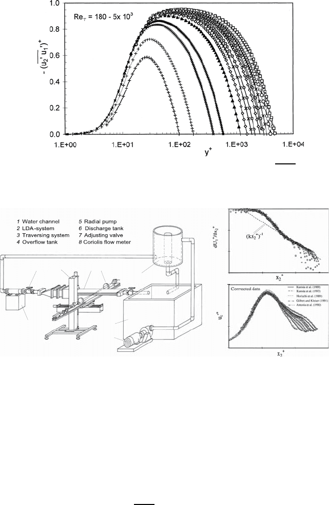
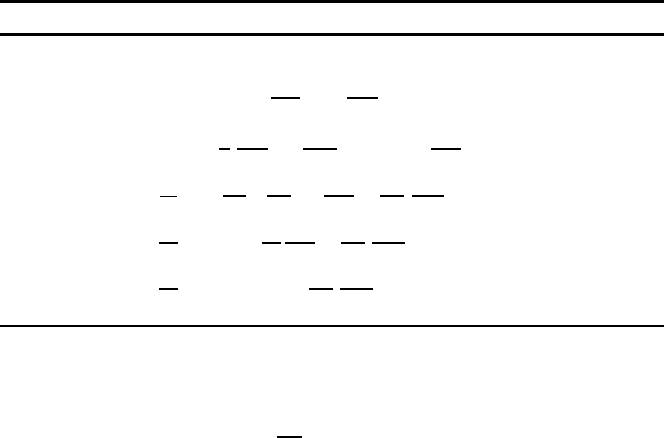
Fig. 18.24 Standardized turbulent momentum transport terms (u



) for plane

channel ﬂows

100 1000

0.001

0.01

0.1

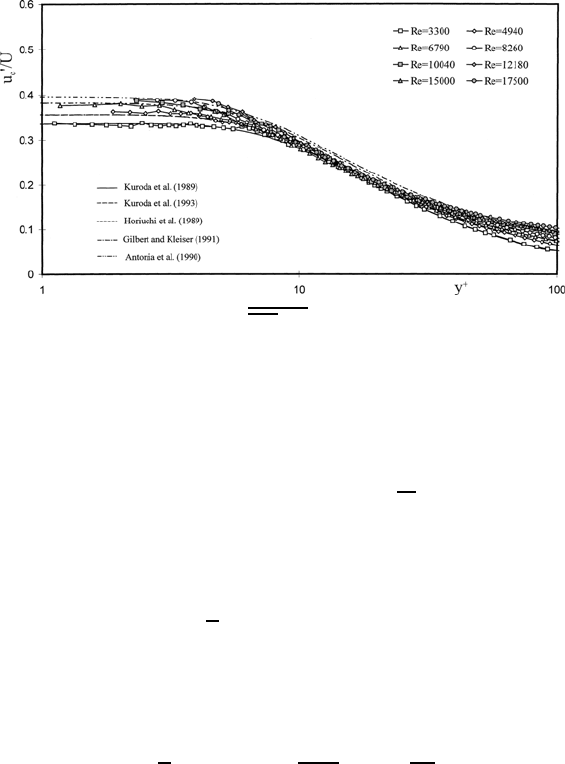
Fig. 18.25 Plane channel ﬂow and LDA system. Measurement results for

standardized turbulent velocity ﬂuctuations in the ﬂow direction

values obtained by numerical investigations, a general trend exists. The re-

maining discrepancies between the experimental and numerical data can, in

all probability, be attributed to mistakes in the numerical computations, as

the computed values were not subjected to corrections concerning the ﬁnite

numerical grid spacings employed.

The investigations described above are limited to such wall roughnesses

for which it holds that

≤  =2.72, (18.246)

i.e. the values κ =1/e and B =10/e are valid only for ﬂows with high

Reynolds numbers and for walls which can be considered to be hydraulically

584 18 Turbulent Flows

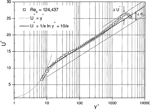
Fig. 18.26 Turbulence intensity





near the wall as a function of the

Reynolds number

smooth. For rough walls, an amendment proves necessary for which the

following considerations hold:

= f(y, ρ, µ, τ

,δ

) ; U

= f





, (18.247)

where δ

represents the “sand roughness” of the wall. Similarity considera-

tions show that the following logarithmic wall law for rough channel walls

can be derived:

ln y

+ B −∆B

. (18.248)

Of particular interest is that point in the viscosity-controlled sub-layer of the

ﬂow where the sub-layer U

= y

and the layer U

=1/κ(ln y

)havethe

same values and the same gradients:

= y

ln y

and

=1=

. (18.249)

From this it follows that at y

= e this consideration is fulﬁlled for κ =1/e,

a value that also resulted from the measurements at LSTM, Erlangen. For

the logarithmic velocity proﬁle with maximum roughness δ

for which a vis-

cosity dominated sub-layer still exists, it results that ∆B(δ

)=B =10/e,

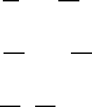
see Fig. 18.27. With this, we can see that a constant representation of the

normalized velocity distributions for hydromechanically smooth and rough

channel walls can be presented. Nevertheless, many questions concerning de-

tailed problems of turbulent wall boundary layers have still to be answered

and need to be investigated with the help of modern measuring and com-

putation techniques. It is especially necessary to extend the results obtained

here for fully developed, two-dimensional, plane, turbulent channel ﬂows to

pipe ﬂows, and also to ﬂat plate ﬂows and turbulent ﬁlm ﬂows.

References 585

Fig. 18.27 Modiﬁcation of the additive constants of the logarithmic wall law due to

roughness

References

18.1. Arpaci, V. S., Larsen, P. S.: “Convection Heat Transfer”, Central Book

Company, Taipei, Taiwan (1984)

18.2. Biswas, G., Eswaran, V.: “Turbulent Flows, Fundamentals, Experiments and

Modeling”, IIT Kanpur Series of Advanced Texts, Narosa Publishing House,

New Delhi (2002)

18.3. Hinze, J. O.: “Turbulence”, 2nd edition, McGraw-Hill, New York (1975)

18.4. Pope, S. B.: “Turbulent Flows”, Cambridge University Press, 2002

18.5. Schlichting, H.: “Boundary Layer Theory”, McGraw-Hill, New York (1979)

18.6. Tennekes, H., Lumley, J. L.: “A ﬁrst Course in Turbulence”, MIT Press,

Cambridge, Mass., USA, (1972)

18.7. Townsend A. A.: “The Structure of Turbulent Shear Flows”, 2nd edition,

Cambridge University Press, Cambridge, UK (1976)

18.8. White, F. M.: “Viscous Fluid Flow”, Kingsport Press, Kingsport (1982)

18.9. Wilcox, D. C.: “Turbulence Modeling for CFD”, DCW Industries, La Canada

(1993)

Chapter 19

Numerical Solutions

of the Basic Equations

∗

19.1 General Considerations

The considerations in Chaps. 13–16 showed that analytical solutions of the

basic equations of ﬂuid mechanics can often only be obtained when simpli-

ﬁed equations or fully developed ﬂows and small or large Reynolds numbers,

respectively, are considered and if, in addition, one limits oneself to ﬂow

problems which are characterized by simple boundary conditions. Even with

these simpliﬁcations, the derivations carried out did not result in analytical

solutions for all ﬂow problems to be solved, but merely reduced the ﬂow de-

scribing partial diﬀerential equations to ordinary diﬀerential equations. As

shown in the previous chapters, the latter could be solved by means of cur-

rent analytical methods. Moreover, the boundary conditions characterizing

the ﬂow problems could also be implemented into these solutions. Thus it was

demonstrated that the methods known in applied mathematics for solving or-

dinary diﬀerential equations represent an important tool for the theoretically

working ﬂuid mechanics researcher. Although analytical techniques for the

solution of ﬂow problems no longer have the signiﬁcance they had in the

past, it is part of a good education in ﬂuid mechanics to teach these methods

to students and for the latter to learn them.

When considering the partial diﬀerential equations discussed in the

preceding chapters, they can all be brought into the subsequent general form

∂

∂x

+2B

∂

∂x∂y

+ C

∂

∂y

+ D

∂Φ

∂x

+ E

∂Φ

∂y

+ FΦ = g(x, y). (19.1)

When designating as the discriminant of the diﬀerential equation (19.1)

d :=AC − B

(19.2)

∗

Important contributions to this chapter were made by my son Dr. -Ing. Bodo

Durst.

587

588 19 Numerical Solutions of the Basic Equations

one deﬁnes the diﬀerential equation as parabolic, hyperbolic or elliptic when

for d the following holds:

Parabolic diﬀerential equation: d = 0 (one-parameter characteristics),

Hyperbolic diﬀerential equation: d<0 (two-parameter characteristics),

Elliptic diﬀerential equation: d>0 (no real characteristics).

This classiﬁcation of the diﬀerential equation orients itself by the equations

for parabolas, hyperbolas and ellipses of the ﬁeld of plane geometry, in which

the equation:

+2bxy + cy

+ dx + ey + f = 0 (19.3)

describes parabolas (ac − b

= 0), hyperbolas (ac − b

< 0) and ellipses

(ac − b

> 0). Accordingly, for the diﬀerential equations discussed in the

preceding chapters, one can characterize:

Diﬀusion equation

∂U

∂t

= ν

∂

∂x

, i.e. it holds A = ν, B = C =0and

thus d = 0. The diﬀusion equation has “parabolic

properties.”

Wave equation

∂

∂t

= c

∂

∂x

, i.e. it holds A = c

, B =0,C =

−1 and thus d = −c

< 0. The wave equation is

hyperbolic.

Potential equation

∂

∂x

∂

∂y

= 0, i.e. A = C =1,B =0andthusd>0.

The potential equation shows “elliptical behavior.”

The stationary boundary-layer equations are, as can be demonstrated

when analyzing them according to the above representations, parabolic diﬀer-

ential equations. Such equations have a property which is important for the

numerical solution to be treated in this section. The solution of the diﬀeren-

tial equation determined at a certain point of a ﬂow ﬁeld, does not depend on

the boundary conditions that lie downstream. This makes it possible to ﬁnd

a solution for the entire ﬂow ﬁeld via “forward integration,” i.e. the solution

can be computed in a certain level of the ﬂow ﬁeld alone from the values of

the preceding level. This is characteristic for parabolic diﬀerential equations

which thus, in the case of numerical integration, possess advantages which

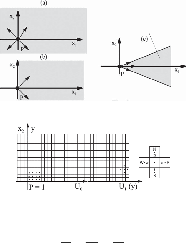
the elliptic diﬀerential equations do not have. This becomes clear when look-

ing at Fig. 19.1, which shows which subdomain of a ﬂow ﬁeld acts on the

properties at a point P , i.e. determines its ﬂow properties.

In order to be able to solve diﬀerential equations numerically, it is necessary

to cover the ﬂow region with a “numerical grid,” as e.g. indicated in Fig. 19.2

for a special ﬂow problem, where a structured grid is shown. This is installed

over a plane plate which carries out the following motion:

=0,t< 0) = 0 The plate rests for all times t<0,

=0,t≥ 0) = U

The plate moves at constant velocity for t ≥ 0.

By the motion of the plate, the ﬂuid above the plate is, due to the molecular

momentum transport, set in motion.

19.1 General Considerations 589

Region of influence of

elliptic diff. equation

Region of influence of

parabolic diff. equation

Region of influence of

hyperbolic diff. equation

Fig. 19.1 Regions of inﬂuence for properties in point P for elliptic (a), parabolic (b)

and hyperbolic (c) diﬀerential equations

Fig. 19.2 Numerical grid for computing the ﬂuid motion for sudden motion of the

plate

The momentum input into the ﬂuid is, assuming an inﬁnitely long plate

in the x

direction, described by the following diﬀerential equation:

∂U

∂t

= ν

∂

∂x

= ν

∂

∂y

. (19.4)

To be able to describe the solution of this diﬀerential equation on the numer-

ical grid of Fig. 19.2, discretizations of the ﬁrst derivative in time and second

derivative in space in the diﬀerential equation (19.4) are necessary. An anal-

ysis of the diﬀerential equation shows that the discriminant is d = 0, i.e. the

diﬀerential equation is parabolic. The solution concerning time t can thus be

computed from the solution concerning time t − ∆t. Inversely it holds, how-

ever, that the solution concerning time (t + ∆t) cannot be used to compute

the solution concerning time t. When using the “ﬁnite-diﬀerence method” for

discretization (see Sect. 19.3), for the time a forward-diﬀerence formulation

590 19 Numerical Solutions of the Basic Equations

and for y a central-diﬀerence formulation can be employed, from which the

following ﬁnite-diﬀerence equation for the diﬀerential equation (19.4) results:

α+1

− U

∆t

= ν

β+1

− 2U

+ U

β−1

(∆y)

. (19.5)

With this the velocity U in the time interval (α + 1) can be computed

explicitly:

α+1

= U

−

ν∆t

(∆y)

β+1

− 2U

+ U

β−1

, (19.6)

i.e. a discrete solution of the diﬀerential equation is possible. The discretized

equation is deﬁned as consistent when for the transition ∆y → 0and∆t → 0

(19.6) turns into the original diﬀerential equation (19.4). Here, checking of the

consistency can be done through an analysis treating the truncation error.

When for ∆y and ∆t → 0 the truncation error heads towards zero, the

employed diﬀerentiation method is consistent.

For the reasonable application of numerical computation methods, it is

moreover necessary that the “discretization method used is stable,” i.e. yields

stable solutions. The required stability is generally guaranteed when perturba-

tions introduced into the solution process are attenuated by the discretization

method. However, when an excitation of occurring perturbations takes place,

the chosen discretization method is deﬁned as unstable. With respect to

ﬂuid-mechanical problems, for stability considerations of the solution meth-

ods employed, the diﬀusion number Di and the Courant number Co are of

importance:

Di =

ν∆t

(∆y)

and Co =

U∆t

∆y

. (19.7)

Here, the diﬀusion number indicates the ratio of the time interval ∆t cho-

sen in the discretization to the diﬀusion time (∆y

)/ν, while the Courant

number states the ratio of the chosen time interval ∆t to the convection

time (∆y/U ). It is understandable that the numerical computation method

can provide stable solutions only when the chosen time intervals ∆t can re-

solve the physically occurring diﬀusion and convection times in the chosen

numerical grid. Details are explained in the subsequent paragraphs.

It is also important for a chosen discretization method that the conver-

gence of the solution is guaranteed. This means that the numerical solution,

with continuous improvements of the numerical grid, agrees more and more

with the exact solution of the diﬀerential equation. Yet the “Lax equiva-

lence theorem” says that stable and consistently formulated discretizations

of linear initial-value problems lead to convergent solutions, i.e. at least for

linear diﬀerential equations, it can be shown that the consistency, stability

and convergence of discretization methods are closely linked properties of a

discretization method employed for the solution of diﬀerential equations. In

the case of existing consistency, it is suﬃcient for a discretization method to

prove its stability, in order to be able to predict reliably its convergence also.

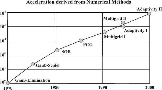
19.2 General Transport Equation and Discretization 591

Fig. 19.3 Increase in performance of mathematical methods for solving basic equa-

tions in ﬂuid mechanics

As far as numerical solutions of the basic equations of ﬂuid mechanics are

concerned, their solution regarding engineering problems is connected to high

computational eﬀorts. By eﬃcient numerical computational methods and the

employment of the currently available high computer power, this can nowa-

days be managed. Developments in applied mathematics have contributed to

this (see Fig. 19.3) and have led to a continuous increase in the performance

of computational methods for numerical solutions of the basic equations of

ﬂuid mechanics. Figure 19.3 shows the increase in performance of numerical

computational methods, which has led, on average, to a tenfold increase ev-

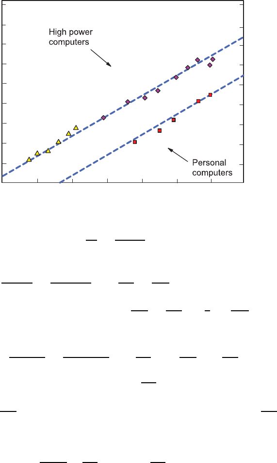
ery 8 years. Combining this with the increase in computational power, which

can be said to have had a tenfold increase every 5 years (see Fig. 19.4), it

becomes understandable why numerical ﬂuid mechanics has been gaining in-

creased signiﬁcance in recent years. It is the ﬁeld of numerical ﬂuid mechanics

to which the greatest importance has to be attached in the near future. The

above increases in computing and computer power have signiﬁcance with re-

gard to solutions of engineering ﬂuid ﬂow problems. It is therefore imperative

that modern ﬂuid-mechanical education has an emphasis on numerical ﬂuid

mechanics. In this chapter, only an introduction to this important ﬁeld can

be given. These are detailed treatments of numerical ﬂuid mechanics given

in refs. [19.1] to [19.6].

19.2 General Transport Equation and Discretization

of the Solution Region

In Chap. 5, the basic equations of ﬂuid mechanics were derived and stated in

the form indicated below:

• Continuity equation:

592 19 Numerical Solutions of the Basic Equations

1940

1950

1970

1960 1980

1990

2000

Univac 1101

IBM 704

Univac Larc

IBM 7030

CDC 7600

Cray - 1S

Cray -2s/4-128

NEC SX -3/44

Intel ASCI Red

8068/87

80386/87

80486

Pentium Pro

2010

AMD K7/600

IBM 701

EDSAC

CYBER205

IntelXP/S140

NEC SX-5/16

Hitachi SR800-F1

Development of computer power (Flop/s)

Fig. 19.4 Increase in the performance of high-speed computers and of personal

computers

∂ρ

∂t

∂ (ρU

)

∂x

=0. (19.8)

• Navier–Stokes equation:

∂ (ρU

)

∂t

∂ (ρU

)

∂x

= −

∂P

∂x

−

∂τ

∂x

+ ρg

(19.9)

= − µ



∂U

∂x

−

∂U

∂x



µδ

∂U

∂x

• Energy equation:

∂ (ρc

T )

∂t

∂ (ρc

T )

∂x

= −

∂q

∂x

− τ

∂U

∂x

− P

∂U

∂x

, (19.10)

= − λ

∂T

∂x

where τ

∂U

∂x

, in the last equation, represents the dissipation and P

∂U

∂x

the work done during expansion. These equations can be transferred into a

general transport equation in such a way that the following equation holds:

∂ (ρΦ)

∂t

∂

∂x



ρU

Φ − Γ

∂Φ

∂x



= S

, (19.11)

where Φ and S

for the diﬀerent equations are indicated in Table 19.1

Considerations on the numerical solution of the basic equations of ﬂuid

mechanics can thus be restricted to equations of the form indicated in (19.11).

19.2 General Transport Equation and Discretization 593

Table 19.1 Φ, Γ and S

values for the general transport equation

Equation ΦΓ S Remarks

Continuity 1 0 0 –

Momentum u

∂

∂x





∂U

∂x



Newtonian ﬂuid and

compressible ﬂow

−

∂

∂x



∂U

∂x



+ g

ρ −

∂P

∂x

Energy T

ρT



∂ν

∂T



−

∂U

∂x

–

−

∂U

∂x

Ideal gas

−

∂U

∂x

Incompressible or

isobaric

The latter comprises a relationship which indicates the variations in terms of

time of (ρΦ) and changes in space in the form of a convection term (ρU

Φ)

and also a diﬀusion term (−Γ

∂Φ

∂x

). In the source term S,allthoseterms

of the considered basic equations are contained that cannot be placed in the

general convection and diﬀusion terms.

With the general transport equation (19.11), a constant description in

terms of time and space is available of all the physical laws to which ﬂuid

motions are subjected. However, the numerical solution of the transport

equation requires a discretization of the equation with respect to time and

space. Thus, through the numerical solutions of ﬂow problems, solutions are

sought only of the ﬂow quantities at determined points in space, which are

arranged at distances of ∆x

. The determination of these points, before start-

ing a numerical solution of a ﬂow problem, is deﬁned as grid generation, i.e.

the entire ﬂow region is subdivided into discrete subdomains. In general, it

is usual to do the subdivision already in such a way that certain advan-

tages result for the sought numerical solution method. Regular (structured)

and irregular (unstructured) grids can, in principle, be employed; experi-

ence shows, however, that the eﬃciency of numerical solution algorithms is

inﬂuenced particularly disadvantageously by the irregularity of the numeri-

cal grid. On the other hand, it holds that in the presence of complex ﬂow

boundaries the grid generation is considerably facilitated by unstructured

grids. Geometrically complex boundaries of ﬂow regions can be introduced

more easily into the numerical computations to be carried out via unstruc-

tured grids. With this, in the case of strongly irregular grids, triangles,

quadrangles, tetrahedrons, hexahedrons, prisms, etc., can be employed in

combination.

Structured grids are characterized by the general property that the neigh-

boring points surrounding a considered grid point correspond to a ﬁrm