Durst F. Fluid Mechanics: An Introduction to the Theory of Fluid Flows
Подождите немного. Документ загружается.

18.3 Statistical Considerations 533
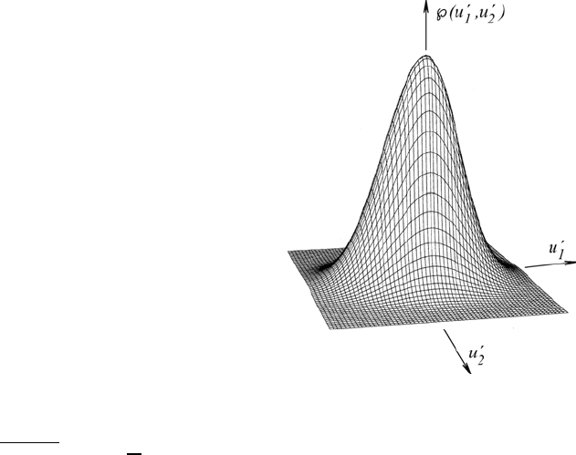
Fig. 18.5 Diagram of a two-dimensional
probability density distribution
u
i
n
u
j
m
= lim
T →∞
1
T
T
#
0
u
i
n
u
j
m
dt =
+∞
#
−∞
u
i
n
u
j
m
℘
!
u
i
,u
j
"
du
i
du
j
. (18.32)
It is again possible to compute these correlations in the time domain of
the velocity field or in the probability density domain. It is important to
emphasize again that the probability density distributions in (18.25), for
the components of the turbulent velocity fluctuation, are probability den-
sity distributions for the turbulent fluctuations at one point in the flow
field.
Two-dimensional probability density distributions ℘(u
1
,u
2
), as shown in
Fig. 18.5, are of special importance in the subsequent treatment of turbu-
lent flows. The above considerations about probability can now be carried
out for two-dimensional functions ℘(u
1
,u
2
), and this results in the following
relationship:
+∞
#
−∞
+∞
#
−∞
℘(u
1
,u
2
)du
1
du
2
=1 and 0≤ ℘(u
1
,u
2
) ≤ 1. (18.33)
When deriving from this two-dimensional distribution the one-dimensional
distribution that applies to the u
1
component of the turbulent velocity field,
i.e. deriving ℘(u
1
), the following relationship holds:
℘(u
1
)=
+∞
#
−∞
℘(u
1
,u
2
)du
2
. (18.34)

534 18 Turbulent Flows
By means of the two-dimensional distribution ℘(u
1
,u
2
), combined moments
of the turbulent velocity components u
1
and u
2
can be computed:
u
1
n
u
2
m
=
#
+∞
#
−∞
u
1
n
u
2
m
℘(u
1
,u
2
)du
1
du
2
. (18.35)
For n = m = 1, the covariance of the velocity components u
1
and u
2
results:
u
1
u
2
=
#
+∞
#
−∞
u
1
u
2
℘(u
1
,u
2
)du
1
du
2
. (18.36)
This integration results in an expression for a correlation existing between
u
1
and u
2
, i.e. it shows to what extent the velocity fluctuations u
1
and u
2
experience correlated changes. Since information of this kind is needed again
and again, for special considerations in the derivations in subsequent sec-
tions, the significance of correlations between turbulent fluctuations will be
explained here briefly. It is important to point out that two turbulent velocity
fluctuations that show no correlation with one another are, in the statistical
sense, not necessarily independent. This becomes clear when one considers
the definitions stated below of independence of two turbulent velocity fluc-
tuations and compares this definition with the condition for the variables to
be uncorrelated:
• Two velocity fluctuations u
1
(t)andu
2
(t) are considered to be statistically
independent when the following relationship for their probability density
distributions holds:
℘(u
1
,u
2
)=℘(u
1
)℘(u
2
), (18.37)
i.e. the probability density of one component of the velocity fluctuations
is not influenced by the distribution of the second.
• Two velocity fluctuations u
1
(t)andu
2
(t) are considered to be uncorrelated
when their covariance is zero, i.e. when the following relationship holds:
u
1
u
2
=
+∞
#
−∞
+∞
#
−∞
u
1
u
2
℘(u
1
,u
2
)du
1
du
2
=0. (18.38)
Two variables are always uncorrelated when the probability density dis-
tribution ℘(u
1
,u
2
) is fully symmetrical, i.e. when it fulfills the following
condition:
℘(+u
1
, +u
2
)=℘(+u
1
, −u
2
)=℘(−u
1
, +u
2
)=℘(−u
1
, −u
2
). (18.39)
Such a symmetrical probability density distribution is shown in Fig. 18.6,
where the isolines ℘(u
1
,u
2
) = constant are shown and lines of equal proba-
bility density. The latter indicate the probability density distribution vertical
to the u
1
− u
2
plane.
18.3 Statistical Considerations 535
Fig. 18.6 Two-dimensional symmetri-
cal probability density distribution with
isolines
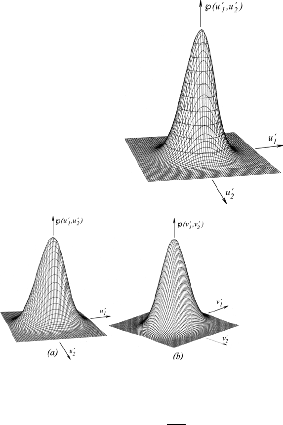
Fig. 18.7 Probability density distribution for isotropic turbulent flows
The probability density distributions shown in Fig. 18.7a, b are identical
with that in Fig. 18.5, but are different in the directions of the coordinate
axes. The latter leads to the finite covariances
v
1
v
2
= 0 indicated in the
figures, i.e. to correlations between v
1
and v
2
. Thus it becomes evident that a
correlation, existing between two turbulent velocity fluctuations is dependent
on the choice of the coordinate system.
For the two coordinate systems indicated in Fig. 18.7 the following holds,
where α is the angle of rotation between the two coordinate systems:
v
1
= u
1
cos α + u
2
sin α,
v
2
= −u
1
sin α + u
2
cos α.
(18.40)
536 18 Turbulent Flows
Using these relationships, one can compute by multiplication and time
averaging:
v
1
v
2
= u
1
u
2
cos 2α − (u
2
1
− u
2
2
)cosα sin α. (18.41)
This relationship makes it clear that
v
1
v
2
is only equal to u
1
u
2
and only equal
to zero when the condition
u
1
2
= u
2
2
is fulfilled (see Fig. 18.6), i.e. when the
flow field is isotropic. By isotropy one understands here a property of the flow
field that shows:
• No directionality of all time-averaged local flow quantities which describe
a turbulent flow field.
In addition, a flow field can have properties which are designated as spatially
homogeneous. For the homogeneity of a flow field, the following holds:
• The time-averaged parameters describing the turbulent flow field are
independent of the position of the measuring location.
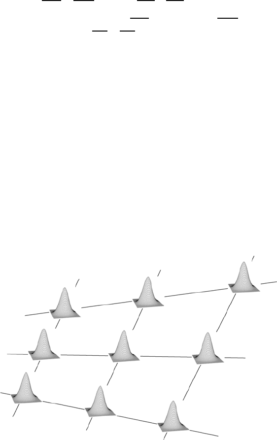
In Fig. 18.8, the two-dimensional probability density distribution of a tur-
bulent isotropic flow field is shown. When the same probability density
distribution exists in each space point and this satisfies the isotropy require-
ments, the turbulence is defined as being homogeneous and isotropic (see
Fig. 18.8).
Fig. 18.8 Spatial distributions of the probability density distributions for isotropic
and homogeneous turbulence
18.3 Statistical Considerations 537
18.3.3 Characteristic Function
For a number of considerations, the Fourier transform of the probability
density distribution is employed, which is usually defined as a characteristic
function of the flow field:
ϕ(k)=
+∞
#
−∞
℘(u
j
)exp(iku
j
(t)) du
j
, (18.42)
where i =
√
−1 represents the imaginary unit of a complex number z = x+iy.
Considering the identity of the operators:
lim
T →∞
1
T
T
#
0
(···)dt =
+∞
#
−∞
(···)p(u
j
)du
j
(18.43)
the characteristic function of the velocity fluctuations u
j
(t) can be computed
as follows:
ϕ(k) = lim
T →∞
1
T
T
#
0
exp(iku
j
(t)) dt. (18.44)
The significance of this function lies, on the one hand, in the experimental
field of turbulence research, where one finds that the convergence of ℘(u
i
)is
bad and that this, with decreasing ∆u
j
, leads to very long measuring times.
The measurement of ϕ(k), on the other hand, is connected to a fairly rapid
convergence and ℘(u
j
) can thus be computed from ϕ(k) as follows (inverse
Fourier transformation):
℘(u
j
)=
+∞
#
−∞
ϕ(k)exp(−iku
j
)dt. (18.45)
The multidimensional characteristic function can also be stated as follows:
ϕ(k
j
) = lim
T →∞
1
T
T
#
0
exp(i{k
j
}{u
j
})dt (18.46)
or by u
j
= {u
1
,u
2
,u
3
} and k
j
= {k, l, m}:
ϕ(k, l,m) = lim
T →∞
1
T
T
#
0
exp[i(ku
1
(t)+lu
2
(t)+mu
3
(t)] dt. (18.47)
538 18 Turbulent Flows
When considering the one-dimensional characteristic function ϕ(k)andits
definition, the following holds:
dϕ
dk
k=0
=
+∞
#
−∞
℘(u
j
)iu
j
du
j
= 0 (18.48)
or quite generally:
d
n
ϕ
dk
n
k=0
= i
n
u
n
j
. (18.49)
The characteristic function enters as a horizontal line into the axis k =0.
At the point k = 0, the derivations of the functions ϕ(k) are linked to the
central moments of the velocity components. Because of this, the character-
istic function can be written as a Taylor series of the corresponding central
moments of the turbulent velocity fluctuations:
ϕ(k)=
∞
n=0
(ik)
n
n!
u
n
i
. (18.50)
These positive properties of the characteristic function can also be put to
very good use in analytical considerations, but in this chapter only its use in
experimental studies is explained.
18.4 Correlations, Spectra and Time-Scales
of Turbulence
In order to obtain information on the structure of turbulence, two different
ways of consideration have gained acceptance, characterized as follows:
• The turbulent velocity fluctuations u
j
(x
i
,t), which in general are functions
of space and time, are usually measured for a fixed location and thus can
be regarded as time series. Information on u
j
(t), for a preset value of x
i
,
is therefore recorded for fixed points in space. Its time-averaged proper-
ties can also be provided in the form of probability density distributions,
characteristic functions, etc.
• The turbulent velocity fluctuations u
j
(x
i
,t) can also be considered for a
fixed time, yielding information on the spatial distributions of the turbu-
lence of the flow field. Information on u
j
(x
i
) is in this way recorded for
fixed points x
i
at the same time t. The entire information on turbulence
can also be provided in the form of two-point probability density distribu-
tions, or multi-point probability density distributions, depending on the
information sought.
18.4 Correlations, Spectra and Time-Scales of Turbulence 539
For considerations of signals varying over time at a fixed point in space,
the question concerning the time interval over which the turbulent velocity
fluctuations are correlated with one another can be answered. This question
can be answered using the autocorrelation function R(τ),whichisdefinedas
follows:
R(τ) = lim
T →∞
1
T
T
#
0
u
i
(t)u
i
(t + τ )dt. (18.51)
With t
= t + τ, the following holds for processes that are stationary in a
time-averaged manner:
u
2
j
(t)=u
2
j
(t
)= constantforτ =0. (18.52)
This constant “effective value” of the turbulent velocity fluctuations can be
employed for the standardization of the autocorrelation function and thus for
the introduction of the autocorrelation coefficient ρ(τ ):
ρ(τ)=
1
u
2
j
R(τ)=
1
u
2
j
lim
T →∞
1
T
T
#
0
u
j
(t)u
j
(t + τ)dt. (18.53)
For the autocorrelation coefficient, the following general properties hold:
ρ(τ)=ρ(−τ) symmetric with the τ =0axis, (18.54)
ρ(0) = 1 and ρ(τ) ≤ 1. (18.55)
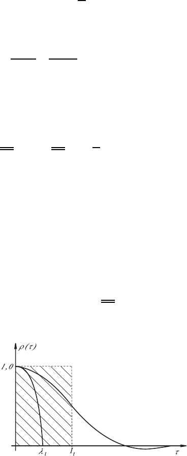
A typical result for ρ(τ) is shown in Fig. 18.9. By means of the autocorrelation
coefficient of a turbulent flow field, through ρ(τ), typical time-scales of tur-
bulence can be introduced. As the integral time-scale the following quantity
is defined:
I
t
=
∞
#
0
ρ(τ)dτ =
1
u
2
j
∞
#
0
R(τ)dτ, (18.56)
Fig. 18.9 Autocorrelation function and time-scales of turbulent velocity fluctuations
540 18 Turbulent Flows
I
t
corresponds, therefore, to the surface below the ρ(τ) distribution, and this
means that the following identity of the surfaces in Fig. 18.9 holds:
u
2
j
I
t
=
∞
#
0
R(τ)dτ. (18.57)
It is a characteristic property of turbulent flows that they show velocity
fluctuations having finite integral time-scales. The integral time-scale I
t
is a
quantity which shows the order of magnitude of the period of time over which
the velocity fluctuations u
j
(t) are correlated with one another. I
t
=0means
that there is no correlation. Such a “degenerated” turbulent flow field cannot
exist in reality; it lacks essential elements for maintaining turbulent flow
fluctuations. Hence, turbulence contains structures of finite time durations.
In fact, turbulent flows contain an entire spectrum of vortex-like structures.
In addition to the integral time-scale of turbulence, a micro time-scale
λ
t
can also be introduced, which is defined through the curvature of the
autocorrelation coefficient function at the point τ =0:
d
2
ρ(τ)
dτ
2
= −
2
λ
2
t
. (18.58)
On expanding ρ(τ) in a Taylor series around τ = 0 and considering the
symmetry of the ρ(τ) distribution, then for the small τ values the following
parabolic function holds:
ρ(τ)=1−
τ
2
λ
2
t
±··· (18.59)
so that by repeated derivatives the above definition equation (18.58) for λ
t
can be derived. Moreover, for the parabola arising from the Taylor series ex-
pansion, it can be derived that this parabola cuts the ρ(τ) = 0 axis (abscissa)
at τ = λ
t
(see Fig. 18.9).
Based on the relationship
d
2
dt
2
u
2
j
=2u
j
d
2
u
j
dt
2
+2
du
j
dt
2
(18.60)
valid for all time-averaged turbulent flow processes which are stationary, we
can derive
d
2
dt
2
u
2
j
=0=2
u
j
d
2
u
j
dt
2
+2
du
j
dt
2
, (18.61)
i.e. the following relationship holds:
du
j
dt
2
= −u
j
d
2
u
j
dt
2
. (18.62)
18.4 Correlations, Spectra and Time-Scales of Turbulence 541
In consideration of the properties of the autocorrelation function, one can
write
du
j
dt
2
=
2
λ
2
t
u
2
j
(18.63)
or, expressed in terms of λ
2
t
:
λ
2
t
=
2
u
2
i
du
i
dt
2
. (18.64)
This shows that the micro time-scale of the turbulence can also be determined
from the double of the rms value of the turbulent velocity fluctuations divided
by the rms value of the time derivative of the turbulent velocity fluctuations.
In conclusion, one should mention, with regard to the above considerations,
that turbulence comprises an entire spectrum of time-scales or corresponding
frequencies, all of which one can imagine to lie in the range between the
integral time-scale I
t
and the micro time-scale λ
t
. This distribution of scales
is determined by the total distribution of the ρ(τ) function which for τ =0has
the value 1, and for all finite τ values the ρ(τ) values satisfy the requirement
ρ(τ) <
1
τ
. (18.65)
As for τ −→ ∞ (18.65) also holds: the integral time-scale can be computed
from ρ(τ) always to have a finite value.
The considerations presented above can also be carried out in the spectral
range. The spectral energy density distribution S(ω) is given as follows:
S(ω)=
+∞
#
−∞
1
2π
ρ(τ)exp{−iωτ} dτ. (18.66)
Thus in reverse, the autocorrelation coefficient S(ω) can be computed from
the spectral energy density distribution by Fourier transformation:
ρ(τ)=
+∞
#
−∞
S(ω)exp{iωτ} dω. (18.67)
For S(0), the following relationship results from the above equation:
S(0) =
+∞
#
−∞
1
2π
ρ(τ)dτ =2
∞
#
0
1
2π
ρ(τ)dτ =
I
t
π
. (18.68)
542 18 Turbulent Flows
With this, the value of the energy spectrum for ω = 0 is determined by the
integral time-scale of the turbulence in the following way:
S(0) =
I
t
π
. (18.69)
The significance of the spectral energy-density distribution also becomes
clear when one considers the Fourier coefficients of the turbulent velocity
fluctuations u
j
(t):
a
T
(ω,t)=
1
T
t+T
#
t
u
j
(t
)exp{iωt
} dt
(18.70)
and the time average of the square of this value:
lim
T →∞
|a
T
(ω,t)|
2
= u
2
i
S(ω). (18.71)
The spectral energy density distribution thus represents the energy of u
j
(t)
at the frequency ω, i.e. the following relationship holds:
dE(ω)
dω
=
u
2
i
S(ω). (18.72)
The total energy can thus be computed as:
E
ges
= u
2
j
∞
#
0
S(ω)dω. (18.73)
18.5 Time-Averaged Basic Equations of Turbulent Flows
It has been stressed in the previous sections that turbulent flows possess com-
plex properties, and one therefore limits oneself to the determination of the
time-averaged properties of turbulent flows, i.e. one does not try to recover the
time-varying properties of the flow field. Because of this, turbulent flows can
therefore be theoretically better treated by the Reynolds equations instead
of the Navier–Stokes equations. In order to derive the Reynolds equations,
the instantaneous velocity
ˆ
U
j
(t) is replaced by the sum of the mean veloc-
ity U
j
and the fluctuation velocity u
j
(t), i.e.
ˆ
U
j
= U
j
+ u
j
and analogously
ˆρ =¯ρ + ρ
,
ˆ
P =
¯
P + p
, etc. Introducing these decomposed quantities into
the Navier–Stokes equations and, by time averaging the equations, a new set
of equations results for the mean values of the flow properties, the so-called
Reynolds equations. The corresponding derivations are shown below.