Durst F. Fluid Mechanics: An Introduction to the Theory of Fluid Flows
Подождите немного. Документ загружается.

420 14 Time-Dependent Flows
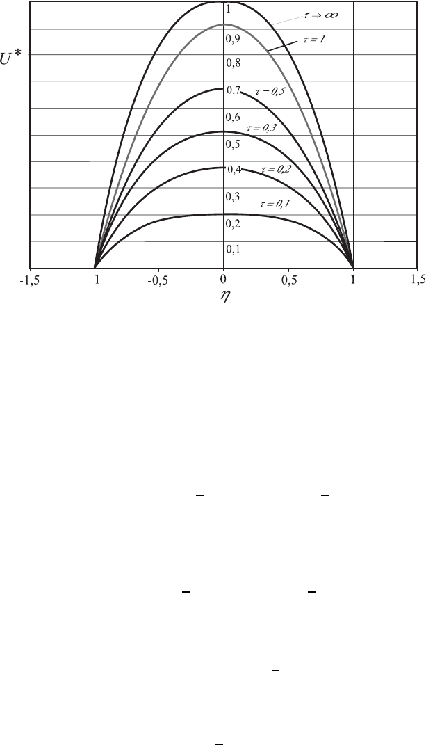
Fig. 14.10 Starting flow between two plane plates according to (14.190)
η, one has to set C = 0. The boundary condition (14.166) applied to (14.172),
takingintoconsiderationC = 0, yields:
0=B cos(λ
n
) (14.173)
This relationship is fulfilled for λ
n
=(n +1/2)π with n =0,±1, ±2, ±3, ···
±∞ so that one obtains as the most general term for the solution of U
∗
t
:
U
∗
t
=
+∞
n=−∞
*
A
n
B
n
exp
3
−
n +
1
2
2
π
2
τ
4
cos
n +
1
2
πη
+
. (14.174)
Considering the symmetry of all n partial functions and setting D
n
=2A
n
B
n
,
(14.174) can be written as:
U
∗
t
=
+∞
n=0
D
n
exp
3
−
n +
1
2
2
π
2
τ
4
cos
n +
1
2
πη
(14.175)
Taking into account the initial condition, one obtains:
1 − η
2
=
+∞
n=0
D
n
cos
n +
1
2
πη
(14.176)
Multiplying both parts of this equation by:
cos
m +
1
2
πη
dη (14.177)
14.4 Pressure Gradient-Driven Fluid Flows 421
one obtains by integration from (−1) to (+1):
#
1
−1
!
1 − η
2
"
cos
m +
1
2
πη
dη = D
m
(14.178)
or, with the following steps of integration:
#
1
−1
cos
m +
1
2
πη
dη −
#
1
−1
η
2
cos
m +
1
2
πη
dη
= D
m
(14.179)
#
1
−1
cos
m +
1
2
πη
dη
=
2sin
!!
m +
1
2
"
π
"
!
m +
1
2
"
π
(14.180)
#
1
−1
η
2
cos
m +
1
2
πη
dη
=
#
u dv = uv −
#
v du (14.181)
u = η
2
⇒ d=2∗ η dη,... dv =cos
m +
1
2
πη
dη ⇒ v =
sin
!!
m +
1
2
"
πη
"
!
m +
1
2
"
π
(14.182)
#
1
−1
η
2
cos
m +
1
2
πη
dη
= η
2
sin
!!
m +
1
2
"
πη
"
!
m +
1
2
"
π
1
−1
−
2
!
m +
1
2
"
π
#
1
−1
η sin
m +
1
2
πη
dη
(14.183)
#
1
−1
η
2
cos
m +
1
2
πη
dη =
2sin
!
m +
1
2
"
π
!
m +
1
2
"
π
−
2
!
m +
1
2
"
π
#
1
−1
η sin
m +
1
2
πη dη (14.184)
#
1
−1
η sin
m +
1
2
πη dη =
#
u dv (14.185)
u = η dv =sin
m +
1
2
πη dη
du =dηv= −
cos
!!
m +
1
2
"
πη
"
!
m +
1
2
"
π
#
1
−1
η sin
m +
1
2
πη dη = −
η cos
!
m +
1
2
"
πη
!
m +
1
2
"
π
1
−1
+
#
cos
!
m +
1
2
"
πη
!
m +
1
2
"
π
dη
=0+
sin
!
m +
1
2
"
πη
7!
m +
1
2
"
π
8
2
1
−1
=
2sin
!
m +
1
2
"
π
7!
m +
1
2
"
π
8
2
(14.186)
422 14 Time-Dependent Flows
D
m
=
2sin
!
m +
1
2
"
π
!
m +
1
2
"
π
−
2sin
!
m +
1
2
"
π
!
m +
1
2
"
π
+
4sin
!
m +
1
2
"
π
7!
m +
1
2
"
π
8
3
(14.187)
sin
m +
1
2
π
=(−1)
m
and cos
m +
1
2
π
=0
Hence, one obtains for D
m
= D
n
:
D
m
⇒ D
n
=
4(−1)
n
!
n +
1
2
"
3
π
3
(14.188)
or for the solution of U
∗
t
:
U
∗
t
=4
+∞
n=0
(−1)
n
!
n +
1
2
"
3
π
3
exp
3
−
n +
1
2
2
π
2
τ
4
cos
n +
1
2
πη
(14.189)
As the complete solution for U
∗
= U
∗
∞
− U
∗
t
,oneobtains:
U
∗
=(1− η
2
) − 4
+∞
n=0
(−1)
n
!
n +
1
2
"
3
π
3
exp
3
−
n +
1
2
2
π
2
τ
4
cos
n +
1
2
πη
(14.190)
or in dimensional quantities:
U
1
=
gD
2
2ν
1 −
x
2
D
2
− 4
+∞
n=0
(−1)
n
!
n +
1
2
"
3
π
3
exp
3
−
n +
1
2
2
π
2
νt
D
2
4
cos
n +
1
2
π
x
2
D
(14.191)
On comparing the above derivations with those that were carried out in
Sect. 14.2.3, it can easily be seen that the derivations correspond to one an-
other. It can now easily be understood that the above derivations for the
starting channel flow are equivalent to those for the fluid flow caused by a
pressure gradient. On replacing the pressure gradient −
dΠ
dx
1
in the deriva-
tions by the gravitational force ρg, all derivations can be transferred to the
pressure-driven channel flow.
14.4.2 Starting Pipe Flow
Another unsteady flow problem is the starting pipe flow, which is of certain
importance in practice. It shall be discussed in this section for those condi-
tions where for t<0 a viscous fluid is at rest in an infinitely long pipe. At
time t = 0 and for all times t ≥ 0, a constant pressure gradient is imposed
on the fluid, i.e. −
∂Π
∂z
is generated along the entire pipe. The flow induced
in this way is described by the partial differential equation
14.4 Pressure Gradient-Driven Fluid Flows 423
∂U
z
∂t
= −
1
ρ
∂Π
∂z
+ ν
1
r
∂
∂r
r
∂U
z
∂r
(14.192)
which was derived for one-dimensional, unsteady flows of incompressible vis-
cous media having a constant viscosity. The initial and boundary conditions
for the starting pipe flow read:
initial conditions: t =0 ; U
z
(r, t)=0for0≤ r ≤ R (14.193)
boundary conditions: r =0 ; U
z
= finally for all t>0 (14.194)
r = R ; U
z
=0forallt>0 (14.195)
One obtains the solution of the considered flow problems by introducing the
following dimensionless variables:
U
∗
z
=
U
z
!
−
∂Π
∂z
"
R
2
4µ
dimensionless velocity (14.196)
η =
r
R
dimensionless position coordinate (14.197)
τ =
µt
ρR
2
dimensionless time (14.198)
so that one has to solve the following differential equation for dimensionless
quantities:
∂U
∗
z
∂τ
=4+
1
η
∂
∂η
η
∂U
∗
z
∂η
(14.199)
The initial and boundary conditions also need to be written for the
dimensionless variables and are:
initial conditions: τ =0 ; U
∗
=0for0≤ η ≤ 1 (14.200)
boundary conditions: η =0 ; U
∗
= finally for τ>0 (14.201)
η =1 ; U
∗
=0forτ>0 (14.202)
To solve the above differential equation, one uses the fact that the considered
flow for τ →∞heads for the laminar, stationary, fully developed pipe flow.
The latter is introduced as a separate partial solution by the solution ansatz,
where one writes U
∗
z
= U
∗
∞
for τ →∞.
The chosen solution ansatz therefore reads for the developing velocity field:
U
∗
(η, τ)=U
∗
∞
(η) − U
∗
t
(η, τ) (14.203)
The stationary part of the solution, i.e U
∗
∞
(η), is obtained by solving the
following differential equation:
0=4+
1
η
d
dη
η
dU
∗
∞
dη
(14.204)
424 14 Time-Dependent Flows
which can be derived from the above partial differential equation (14.199) by
setting
∂U
∗
∂τ
=0 for τ →∞. By integration one obtains:
U
∗
∞
(η)=−η
2
+ C
1
ln η + C
2
(14.205)
Employing the boundary conditions, one obtains for the integration constants
C
1
=0andC
2
= 1 and thus for U
∗
∞
the following results:
U
∗
∞
(η)=1− η
2
(14.206)
Hence the Hagen–Poiseuille velocity distribution of the fully developed pipe
flow is obtained.
On inserting now U
∗
∞
=1−η
2
into the differential equation (14.203), one
obtains:
U
∗
(η, τ)=(1− η
2
) − U
∗
t
(η, τ) (14.207)
By insertion of this relationship into the differential equation (14.199), the
following differential equation can be derived:
−
∂U
∗
t
∂τ
=4+
1
η
∂
∂η
η
∂
∂η
!
1 − η
2
"
−
1
η
∂
∂η
η
∂U
∗
t
∂η
(14.208)
or, after having carried out the differentiations:
∂U
∗
t
∂τ
=
1
η
∂
∂η
η
∂U
∗
t
∂η
(14.209)
This differential equation now has to be solved for the following initial and
boundary conditions:
initial conditions: τ =0; U
∗
t
(η, 0) = U
∞
(η)for0≤ η ≤ 1 (14.210)
boundary conditions: η =0; U
∗
t
= finite for all τ>0 (14.211)
η =1; U
∗
t
=0forallτ>0 (14.212)
Again, a separation ansatz for the variables η and τ is employed for solving
the differential equation for U
∗
t
:
U
∗
t
= f(η)g(τ) (14.213)
This ansatz leads to the following relationship:
1
g
dg
dτ
=
1
f
1
η
∂
η
η
df
dη
= −λ
2
(14.214)
Hence it is necessary to solve the following differential equations for g and f:
dg
dτ
= −λ
2
g (14.215)

14.4 Pressure Gradient-Driven Fluid Flows 425
and
1
η
d
dη
η
df
dη
+ λ
2
f = 0 (14.216)
These are differential equations known in the field of unsteady fluid
mechanics. Their solutions are known and can be stated as follows:
g = A exp(−λ
2
τ) (14.217)
f = BJ
0
(λη)+CY
0
(λη) (14.218)
In these general partial solutions of the differential equations (14.215) and
(14.216), the quantities J
0
(λη)andY
0
(λη) are Bessel functions of the first
and second kind of zero order. A, B and C are integration constants which
have to be determined by the initial and boundary conditions for U
∗
t
(η, τ).
When employing the first boundary condition (14.211), i. e. η =0; U
∗
t
is
finite, one obtains C =0,sinceY
0
(0) = −∞. Hence, one obtains for U
∗
t
:
U
∗
t
= A exp(−λ
2
τ)BJ
0
(λη) (14.219)
If one demands that the second boundary condition (14.212) be fulfilled, i.e.
U
∗
t
=0forη =1,thenJ
0
(λ) = 0 has to be fulfilled and only those λ
values are permissible that fulfil these conditions. The following values can
be computed:
λ
1
=2, 405; λ
2
=5, 520; λ
3
=8, 654; etc. (14.220)
i.e. there is a large number of discrete flows, one for each value of λ
n
,which,
summed up, result in the following general solution:
U
∗
t
=
∞
n=1
A
n
exp(−λ
2
n
τ)J
0
(λ
n
η) (14.221)
This general solution now fulfils the partial differential equation which de-
scribes the flow problem and the characteristic boundary conditions. Fulfilling
the flow condition can now serve to determine the integration constant A
n
,
not yet defined. For τ → 0, the following holds:
(1 − η
2
)=
∞
n=1
A
n
J
0
(λ
n
η) (14.222)
When one multiplies both sides of this equation by:
J
0
(λ
m
η)η dη (14.223)
and integrates from 0 to 1, i.e. when one carries out the following arithmetic
operations in the subsequent equation:
1
#
0
J
0
(λ
m
η)(1 − η
2
)η dη =
∞
n=1
A
n
1
#
0
J
0
(λ
n
η)J
0
(λ
m
η)η dη (14.224)
426 14 Time-Dependent Flows
one obtains, because of the orthogonality of the Bessel function, values of the
right-hand side that are different from zero only when m = n.Onemploying
known relationships for the Bessel functions, one obtains:
4J
1
(λ
n
)
λ
3
n
= A
n
1
2
[J
1
(λ
n
)]
2
(14.225)
or, rewritten,
A
m
=
8
λ
3
m
J
1
(λ
m
)
(14.226)
Hence one can deduce for U
∗
t
U
∗
t
=8
∞
n=1
J
0
(λ
n
η)
λ
3
n
J
1
(λ
n
)
exp
!
−λ
2
n
τ
"
(14.227)
and for the total velocity
U
∗
=
!
1 − η
2
"
− 8
∞
n=1
J
0
(λ
n
η)
λ
3
n
J
1
(λ
n
)
exp
!
−λ
2
n
τ
"
(14.228)
The velocity distributions computed according to (14.228) are shown in
Fig. 14.11, where the development of the velocity profile can be seen. Again,
for (νt/R
2
) = 1 the fluid flow has reached the stationary state of fully
developed laminar pipe flow with an accuracy that is sufficient in practice.
Again, similar to chapter 13, only some examples of time-dependent, one-
dimensional flows are treated in this chapter. Further, treatments are found
in refs. [14.1] to [14.6]
Pipe wall
Centre of pipe
Fig. 14.11 Velocity distribution in the pipe for the starting, pressure-driven laminar
pipe flow
References 427
References
14.1. Bird, R.B., Stewart, W.E., Lightfoot, E.N., “Transport Phenomena”, Wiley,
New York, 1960
14.2. Bosnjakovic, R., “Technische Thermodynamik”, Theodor Steinkopf Verlag,
Dresden, 1965
14.3. Eckert, E.R.G., Drake, R.M., Jr., “Analysis of Heat and Mass Transfer”,
McGraw-Hill Kogakusha, Tokyo, 1972
14.4. Sherman, F.S., “Viscous Flow”, McGraw-Hill, Singapore, 1990
14.5. Stokes, G.G., “On the Effect of the Internal Friction of Fluids on the Motion
of Pendulums”, Cambridge Philosophical Transactions IX, 8, 1851
14.6. Stokes, G.G., “Mathematical and Physical Papers”, Cambridge Philosophical
Transactions III, 1–141, 1901

Chapter 15
Fluid Flows of Small Reynolds Numbers
15.1 General Considerations
As shown in the preceding chapters of this book, the integrations of the
generally valid basic equations of fluid mechanics, that were derived in differ-
ential form in Chap. 5, are only successful, by means of analytical methods,
when simplifications concerning the dimensionality of the considered flows
are made. Furthermore, one has to choose for the treatment of transport
problems in fluids very simple boundary conditions. These simple bound-
ary conditions correspond to simple flow problems. For analytical solutions,
they often have to be chosen in such a simple way, that the insights into
the physics of fluid flows resulting from the solutions are of only slight
practical interest. In general, this means that practically relevant flow prob-
lems cannot be treated by analytical solutions of the generally valid basic
equations of fluid mechanics. The boundary conditions, which have to be
imposed on the solutions, are mostly so complicated for practically interest-
ing flows, that they can only be implemented in analytical solutions to some
extent. Thus, fluid mechanics researchers, interested in analytical solutions,
have only the possibility to treat such flow problems, for which the basic
equations can be simplified. The solution of these equations often means
that the considerations still have also to be restricted to flows with sim-
ple geometries, e.g. the flow around spheres, or the flow around cylinders.
To study flows of this kind, the considerations start from the general basic
equations that have been made dimensionless with the inflow velocity U
∞
,
a geometric dimension D, the fluid density ρ, the fluid viscosity µ,etc.This
yields
ρ
∗
D
t
c
U
∞
∂U
∗
∂t
∗
+ U
∗
i
∂U
∗
j
∂x
∗
i
= −
∆P
c
ρU
2
∞
∂P
∗
∂x
∗
j
+
µ
ρU
∞
D
µ
∗
∂
2
U
∗
j
∂x
∗
i
2
+
gD
U
2
∞
ρ
∗
g
∗
j
(15.1)
429
430 15 Fluid Flows of Small Reynolds Numbers
or, rewritten with St = D/(t
c
U
∞
) (Strouhal number), Eu = ∆P/(ρU
2
∞
)
(Euler number), Re =(U
∞
D)/ν (Reynolds number) and Fr = U
2
∞
/(gD)
(Froude number):
ρ
∗
St
∂U
∗
j
∂t
∗
+ U
∗
i
∂U
∗
j
∂x
∗
i
= −Eu
∂P
∗
∂x
∗
j
+
1
Re
µ
∗
∂
2
U
∗
j
∂x
∗
i
2
+
1
Fr
ρ
∗
g
∗
j
. (15.2)
For stationary flows that are not influenced by gravitational forces, and where
the viscosity forces are larger than the acceleration forces, i.e. for Re < 1,
the following reduced form of the momentum equation can be employed:
Eu
∂
2
P
∗
∂x
∗
j
2
+
1
Re
µ
∂
2
U
∗
j
∂x
∗
i
2
=0 ; 0=−
∂P
∂x
j
+ µ
∂
2
U
j
∂x
i
2
(j =1, 2, 3).
(15.3)
This simplification of the momentum equation is valid for such flows that
have the following properties:
• The geometric dimensions of the bodies are small, around which flow takes
place, or the channels are small in which flows occur.
• Flows characterized by very small flow velocities (creeping flows).
• Flows of fluids with large coefficients of kinematic viscosity.
When all the above requirements for a flow are present at the same time,
one arrives at conditions for the presence of smallest Reynolds numbers, i.e.
at flows, where the fluid flows are characterized by viscous length, time and
velocity scales. This will be explained at the end of the present chapter, where
the properties of creeping flows are treated.
The differential equations given in Chap. 5, the continuity and the Navier–
Stokes equations, read for Re → 0:
∂U
i
∂x
i
=0 and 0=−
∂P
∂x
j
+ µ
∂
2
U
j
∂x
i
2
. (15.4)
These are known as the Stokes equations. For two-dimensional, fully devel-
oped flows they are identical with the equations discussed in Chap. 13, when
g
j
is set equal to zero. In this respect, some of the flows treated in this chapter
are related to those in Chap. 13. This fact is pointed out at the appropriate
place in the treatment of creeping flows.
By attempting the treatment of simplified forms of the basic equations,
multidimensional flow problems can be included in the analytical treatment
of flows. This will be shown with examples in Sects. 15.2–15.8. These exam-
ples have been chosen in such a way that they demonstrate, on the one hand,
the multidimensionality of the possible computations achievable by simplifi-
cations and, on the other, the employment of the basic equations to practical
flow problems of small Reynolds numbers. The fluid mechanics of slide bear-
ings are considered. In addition, the rotating flow around a cylinder and the
rotating flow around a sphere are discussed. For both geometries, the transla-
tory motions and the rotating motions are considered. These considerations