Durst F. Fluid Mechanics: An Introduction to the Theory of Fluid Flows

Подождите немного. Документ загружается.

268 9 Stream Tube Theory

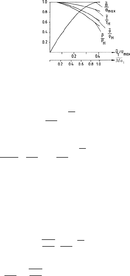
Fig. 9.11 Distribution of the pres-

sure, density, temperature and mass

ﬂow density for converging nozzles

Figure 9.11 also contains the distribution of the ﬂux density θ =˙m/A =˜ρ

i.e. the mass ﬂowing per unit area and unit time through the cross-section of

the ﬂow. The equation for this quantity can be written as follows, using the

relationships for

and ˜ρ:

˜ρ

= ρ

⎡

⎣

1 −

max

⎤

⎦

κ−1

(9.90)

or for the normalized mass ﬂow density:

˜ρ

max

⎡

⎣

1 −

max

⎤

⎦

κ−1

(9.91)

The above relationship for the mass ﬂow density makes it clear that for

= 0, the mass ﬂow θ = 0 is achieved. The mass ﬂow density, however,

assumes the value zero also for U

= U

max

. The reason for this is that at

the maximum possible velocity the density of the ﬂuid, also determining the

mass ﬂow density, has dropped to ˜ρ = 0. Between these two minimum values

the mass ﬂow density has to traverse a maximum which can be computed by

diﬀerentiation of the above functions and by setting the derivation to zero.

The value obtained by solving the resulting equation has to be inserted for

max

in the above equation for the mass ﬂow density in order to achieve

the maximum value. We have:

max

= ρ

max

κ − 1

κ +1



κ +1



κ−1

(9.92)

where for the velocity value:

max

κ − 1

κ +1

for θ = θ

max

(9.93)

9.4 Compressible Flows 269

With this, the mass ﬂow density normalized with the maximum value can be

written as:

max

κ +1

κ − 1

max

κ +1

1 −

max

κ−1

(9.94)

The distribution of this quantity with

max

is also represented in Fig. 9.10.

The signiﬁcance of the maximum of the mass ﬂow density for the distribution

of pressure-driven ﬂows is dealt with more in detail later. Its appearance

prevents a steady increase of the mass ﬂow with increase in the pressure

diﬀerence between the pressure reservoirs when the compensating ﬂow takes

place via steadily converging nozzles.

A representation of the ﬂows through converging nozzles, often regarded as

simpler, is achieved by relating the quantities designating the ﬂow to the cor-

responding quantities of the “critical state”, which is designated by Ma =1.

To this state corresponds not only a certain Mach number, i.e.

=1,

but also certain values of the thermodynamic state quantities: These can be

determined from (9.87)–(9.89) by setting

= 1. From this the following

values for thermodynamic state quantities of the ﬂuid result at the critical

state of the ﬂow, i.e. for

=1:

∗



κ +1



κ−1

(9.95)

˜ρ

∗



κ +1



κ−1

(9.96)

∗

κ +1

(9.97)

With these equations, the pressure, density and temperature of a ﬂowing

medium can be determined in that cross-section of a converging nozzle in

which the velocity of the ﬂuid takes on the local sound velocity. According to

the considerations at the end of Sect. 9.4.1, a minimum of the cross-section has

to exist at this point. As here the Mach number assumes the value

=1,

(9.83) can be written as follows:

∗2

max

κ − 1

κ +1

(9.98)

On comparing the values for

max

in 9.98 and 9.93, one ﬁnds that they are

identical, i.e. the maximum mass ﬂow density can only occur in the narrowest

cross-section of a nozzle, where the sound velocity then also applies.

In accordance with the above derivations of the basic equations for

pressure-driven ﬂows between large reservoirs, the ﬂow which occurs in a

steadily converging nozzle, as sketched in Fig. 9.7, will be discussed. The

270 9 Stream Tube Theory

considerations will be carried out in such a way that the mass ﬂow is com-

puted which results when a certain pressure relationship (P

) between

the reservoirs applies. Here two pressure ranges are of interest:

∗

The ratio of the normalized reservoir pressures is

larger than the critical pressure ratio

∗

The ratio of the reservoir pressures is smaller than

the critical pressure ratio

When the pressure ratio is larger than the critical value, a steady decrease

in the ratio of the reservoir pressures leads to a steady increase in the mass

ﬂow density, as indicated in Fig. 9.11. The latter represents part of the total

diagram stated in Fig. 9.10, namely up to Ma = 1. For the variation of the

state quantities, namely for the pressure and the density the diagram is given.

On the assumption that in the narrowest cross-section of the steadily con-

verging nozzle the pressure of the low-pressure reservoir sets in, the pressure

ratio P

can be determined from the known values P

and P

.Viathe

same approach the mass ﬂow density in this cross-section can be determined

in the following manner and thus also the total mass ﬂowing through the

nozzle:

˙m

= A

(˜ρ

)

(9.99)

For reasons of continuity, this total mass ﬂow is constant in all cross-section

planes of the nozzle, so that

˙m

=˙m i.e. A

= A

(9.100)

Starting from the assumption that the speciﬁed distribution of the cross-

sectional area of the nozzle along the x

axis is known, then the mass ﬂow

density distribution along the x

axis can be determined using (9.100). Via

the same approach, one can then compute, as indicated in Fig. 9.12, the

pressure distribution along the nozzle, or the resulting distributions of the

density and the temperature, but also of the Mach number and the ﬂow

velocity.

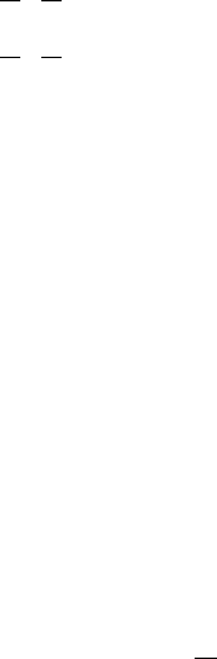
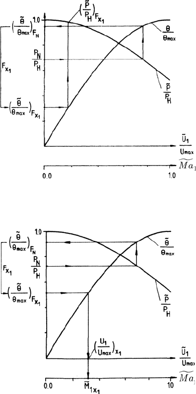
The approach to determining the pressure distribution along the nozzle,

indicated in Fig. 9.13, can be applied analogously also to deﬁne the density

distribution and the temperature distribution. To determine the distribution

of the Mach number and the velocity, the approach indicated in Fig. 9.12

holds.

It follows from the above considerations that the velocity (U

)

in the

entrance cross-section of the nozzle indicated in Fig. 9.7 is ﬁnite and that

there the mass ﬂow density



˜ρ



(9.101)

9.4 Compressible Flows 271

Fig. 9.12 Determining the pressure distribution along the nozzle axis for

) > (P

∗

)

Fig. 9.13 Determining the Mach number and the velocity distribution along a

converging nozzle for (P

) < (P

∗

)

is present. Also in this cross-section a pressure, a density and a temperature

exist which do not correspond to the values in the high-pressure reservoir. It

is necessary always to take this into consideration when computing pressure-

driven ﬂows through nozzles. The quantities designating the ﬂows that exist

at the nozzle entrance are to be determined via the above diagrams from the

mass ﬂow density computed for the entrance cross-section in accordance with

(9.101).

272 9 Stream Tube Theory

When carrying out the above computations for determining the ﬂow quan-

tities and the thermodynamic quantities, with a decrease in the pressure ratio

an increase in the mass ﬂow density in each cross-section of the nozzle

is obtained, as long as the pressure ratio is larger than the critical value. When

the critical value itself is reached:



κ +1



κ−1

∗

(9.102)

This value cannot be exceeded in the case of a further decrease in the pressure

ratio P

i.e. for all pressure ratios smaller than the critical value:

∗



κ +1



κ−1

(9.103)

in the steadily converging nozzle, a ﬂow comes about which is identical

for all pressure relationships. At the exit cross-section of the nozzle, i.e. in

the entrance cross-section to the low-pressure reservoir, the pressure P

longer applies. In this cross-section, the maximum mass ﬂow density rather

is reached:

max

= ρ

2κ

κ − 1

2κ

κ − 1

(9.104)

max

= ρ



(9.105)

The total mass ﬂow thus is computed as:

˙m =˙m

max

= A

max

(9.106)

Starting again from the assumption that the nozzle form is known, then

the mass ﬂow distribution existing along the axis x

can be computed via

the continuity equation. When this distribution is known, the corresponding

distributions of the pressure, density, temperature, Mach number and ﬂow

velocity can be determined as stated above. Of importance is that for all

pressure ratios P

that are equal to or smaller than the critical ratio,

the same ﬂow occurs in the nozzle. In the exit cross-section of the nozzle for

∗



κ +1



κ−1

(9.107)

an area-averaged pressure exists which is larger than the pressure P

existing

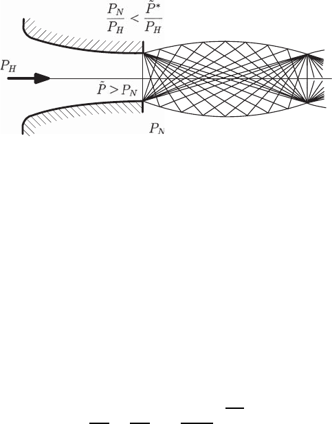
in the low-pressure reservoir. The pressure compensation takes place via ﬂuid

ﬂows that form in the open jet ﬂow, stretching from the nozzle tip to the

interior of the low-pressure reservoir (Fig. 9.14).

Finally, attention is drawn to important facts that arise when considering

pressure-driven ﬂow. The above representations started from the state often

References 273

Fig. 9.14 Pressure compensation at the nozzle exit via density impacts

existing in practice that pressure-driven ﬂows are controlled via pressure dif-

ferences between reservoirs. This means that it was assumed that P

,ρ

are known and constant and that they have an inﬂuence on how the ﬂow

forms. In the low-pressure reservoir it was only assumed that P

is given and

can be forced upon the ﬂow in the narrowest cross-section of the nozzle (for

larger than the critical value P

∗

). The density of the ﬂowing gas

that occurs for these conditions in the exit cross-section of the nozzle or the

temperature that arises are not identical with the corresponding values for

the ﬂuid in the low-pressure reservoir.

Equalization of these values and the corresponding values for the low-

pressure reservoir takes place in the open jet ﬂow following the nozzle ﬂow.

For pressure conditions

∗



κ +1



κ−1

(9.108)

the equalization takes place between the pressure in the nozzle exit cross-

section and the pressure in the low-pressure reservoir, and likewise in the

open jet ﬂow following the nozzle ﬂow. Further details of one-dimensional

compressible ﬂows are provided in refs. [9.1] to [9.2].

References

9.1. E. Becker: “Technische Thermodynamik”, Teubner Studienbuecher Mechanik,

B.G. Teubner, Stuttgart (1985)

9.2. K. Hutter: “Fluid- und Thermodynamik - Eine Einfuehrung”, Springer, Berlin

Heidelberg New York (1995)

9.3. K. Oswatitsch: “Gasdynamik,” Springer, Berlin Heidelberg New York (1952)

9.4. J.H. Spurk: “Stroemungslehre”, 4. Auﬂage, Springer, Berlin Heidelberg New

York (1996)

9.5. S.W. Yuan: “Foundations of Fluid Mechanics”, Civil Engineering and Mechanics

Series, Mei Ya Publications, Taipei, Taiwan (1971)

Chapter 10

Potential Flows

10.1 Potential and Stream Functions

In order to make the integration of the partial diﬀerential equation of ﬂuid

mechanics possible by simple mathematical means, the introduction of irro-

tationality of the ﬂow ﬁeld is necessary. The introduction of irrotationality is

necessary to yield a replacement for the momentum equations and it is this

fact that permits simpler mathematical methods to be applied. In Sect. 5.8.1,

a transport equation equivalent to the momentum equation was derived for

the vorticity which for viscosity-free ﬂows is reduced to the simple form

Dω/Dt = 0. From this equation, two things follow. On the one hand, it

becomes evident that irrotational ﬂuids obey automatically a simpliﬁed form

of the momentum equation. On the other hand, Kelvin’s theorem results im-

mediately, according to which all ﬂows of viscosity-free ﬂuids are irrotational,

when at any point in time the irrationality of the ﬂow ﬁeld was detected. This

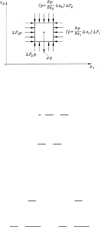
can be understood graphically by considering that all surface forces acting on

a non-viscous ﬂuid element act normal to the surface and as a resultant go

through the center of mass of the ﬂuid element. At the same time, the inertia

forces also act on the center of mass, so that no resultant momentum comes

about which can lead to a rotation. Hence the conclusion is possible that

rotating ﬂuid elements cannot receive an additional rotation due to pressure

and inertia forces acting on ideal ﬂuids. This is indicated in Fig. 10.1.

In addition to the above requirement for irrotationality, a further restric-

tion will now be introduced regarding the properties of the ﬂows that are dealt

with in this chapter, namely the exclusive consideration of two-dimensional

ﬂows. This restriction imposed on the allowable properties of ﬂows is not a

condition resulting from irrotationality; one can, on the contrary, well imagine

three-dimensional ﬂows of viscosity-free ﬂuids that are irrotational. For two-

dimensional, irrotational ﬂows there exists, however, a very elegant solution

method which is based on the employment of complex analytical functions

and which is used exclusively in the following.

275

276 10 Potential Flows

Fig. 10.1 Graphical representation of the physical cause of irrotationality of ideal

ﬂows (Kelvin’s theorem)

When considering two-dimensional ﬂow ﬁelds with ﬂow property de-

pendences on x

and x

, the only remaining component of the rotational

vector is:



∂U

∂x

−

∂U

∂x



. (10.1)

When one assumes the considered two-dimensional ﬂow ﬁelds to be

irrotational, it holds that ω

=0or:

∂U

∂x

∂U

∂x

. (10.2)

This condition has to be fulﬁlled in addition to the continuity equation when

irrotational two-dimensional ﬂow problems are to be solved.

Disregarding singularities, for irrotational ﬂow ﬁelds the above relation-

ship has to be fulﬁlled in all points of the ﬂow ﬁeld. This is tantamount to

the statement that, for two-dimensional irrotational ﬂows, a velocity poten-

tial Φ(x

) driving the ﬂow exists, to such an extent that the following

relationships hold:

∂Φ

∂x

and U

∂Φ

∂x

. (10.3)

Equation (10.3) inserted in (10.2) leads to the following relations:

∂U

∂x

∂

∂x

and

∂U

∂x

∂

∂x

, (10.4)

which for irrotational ﬂow ﬁelds, i.e. for ω

= 0 [see (10.1)], conﬁrm the

reasonable introduction of a potential driving the velocity ﬁeld. When one

10.1 Potential and Stream Functions 277

inserts (10.3) into the two-dimensional continuity equation (5.18) for ρ =

constant then one obtains the Laplace equation for the velocity potential:

∂

∂x

∂

∂x

=0. (10.5)

For determining two-dimensional potential ﬁelds, it is suﬃcient to solve

(10.3) and (10.5), i.e. for determining the velocity ﬁeld it is not necessary to

solve the Navier–Stokes equation, formulated in velocity terms. These equa-

tions, or the equation derived in Sect. 5.8.1, have to be employed, however,

for determining the pressure ﬁeld.

The solution of the partial diﬀerential (10.5) for the velocity potential

requires at the boundary of the ﬂow the boundary condition

∂Φ

∂n

=0, (10.6)

where n is the normal unit vector at each point of the ﬂow boundary.

When the velocity potential Φ, or potential ﬁeld Φ, has been obtained as

a solution of (10.5), the velocity components U

and U

can be determined

for each point of the ﬂow ﬁeld by partial diﬀerentiations, according to (10.3).

After that, the determination of the pressure via Euler’s equations, i.e. via the

momentum equations for viscosity-free ﬂuids, can be computed. Determining

the pressure can also be done, however, via the integrated form of Euler’s

equations, which leads to the “non-stationary Bernoulli equation”.

The above treatments make it clear that the introduction of the irrotation-

ality of the ﬂow ﬁeld has led to considerable simpliﬁcations of the solution

ansatz for the basic equations for ﬂow problems. The equations that have to

be solved for the ﬂow ﬁeld are linear and they can be solved decoupled from

the pressure ﬁeld. The linearity of the equations to be solved is an essential

property as it permits the superposition of individual solutions of the equa-

tions in order to obtain also solutions of complex ﬂow ﬁelds. This solution

principle will be used extensively in the following sections.

In the derivations of the above equations for two-dimensional potential

ﬂows, the potential function was introduced in such a way that the irro-

tationality of the ﬂow ﬁeld was fulﬁlled by deﬁnition. The introduction of

the potential function Φ into the continuity equation then led to the two-

dimensional Laplace equation; only such functions Φ which fulﬁl this equation

can be regarded as solutions of the basic equations of irrotational ﬂows.

Via a procedure similar to the above introduction of the potential function

Φ, it is possible to introduce a second important function for two-dimensional

ﬂows of incompressible ﬂuids, the so-called stream function Ψ . The latter is

deﬁned in such a way that through the stream function the two-dimensional

continuity equation is automatically fulﬁlled, i.e.

∂Ψ

∂x

and U

= −

∂Ψ

∂x

. (10.7)

278 10 Potential Flows

This relationship, inserted into the continuity equation, shows directly that

the stream function Ψ (introduced according to (10.7)) fulﬁlls this equation;

by deﬁnition this is the case for rotational and irrotational ﬂow ﬁelds.

When one wants to deﬁne analytically or numerically the stream function

of an irrotational ﬂow the function Ψ has to be a solution of the Laplace

equation:

∂

∂x

∂

∂x

=0. (10.8)

This equation can be derived by inserting equations (10.7) into the condition

for the irrotationality of the ﬂow:

∂U

∂x

−

∂U

∂x

=0.

The stream function for two-dimensional potential ﬂows fulﬁls the two-

dimensional Laplace equation, similar to the potential function Φ.

The stream function has a number of properties that prove useful for

the treatment of two-dimensional ﬂow problems. Lines of constant stream-

function values, for example, are path lines of the ﬂow ﬁeld when stationary

conditions exist for the ﬂow. This can be derived by stating the total

diﬀerential of Ψ:

dΨ =

∂Ψ

∂x

∂Ψ

∂x

. (10.9)

For Ψ = constant dΨ = 0 and therefore





Ψ =constant

= −

∂ψ

∂x

∂Ψ

∂x

. (10.10)

This is the relationship for the gradient of the tangent of the stream line,

but also for the gradient of the path line of a ﬂuid element. Accordingly, the

total family of stream lines of a velocity ﬁeld is described by all of Ψ values

from 0 to inﬁnity.

A further essential property of the stream function becomes clear from

the fact that the diﬀerence of the stream-function values of two ﬂow lines

indicates the volume ﬂow rate that ﬂows between the ﬂow lines. This can

be derived with the aid of Fig. 10.2, which shows two ﬂow lines that are

connected to one another by a control line AB.

When computing the volume ﬂow that passes the control area AB in the

ﬂow direction passing perpendicular to the x

− x

plane of depth 1, one

obtains:

Q =

−

− U

). (10.11)