Ames W.F., Roger C. Nonlinear equations in the applied sciences. Volume 185
Подождите немного. Документ загружается.

300
Greg
King
and
Ian
Stewart
a
Q
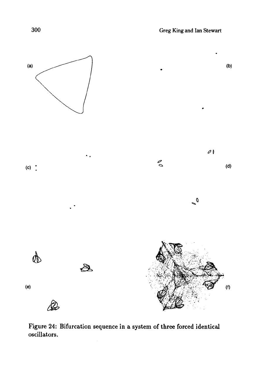
Figure
24:
Bifurcation sequence in a system of three forced identical
oscillators.
Symmetric
Chaos
301
.
*.-
;
,...
I:
;P-'
.
..
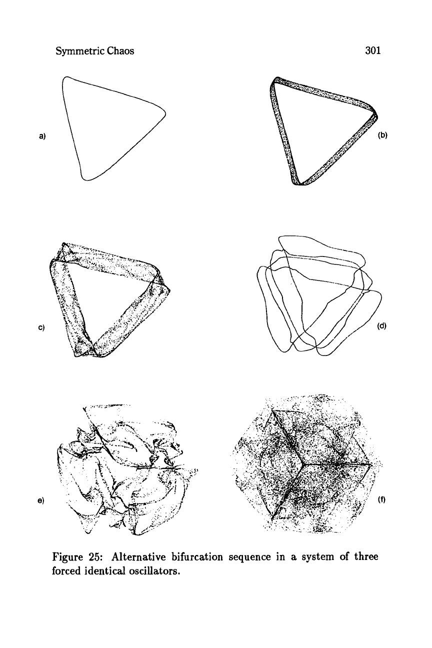
Figure
25:
Alternative bifurcation sequence in
a
system
of
three
forced identical oscillators.
302
Greg
King
and
Ian
Stewart
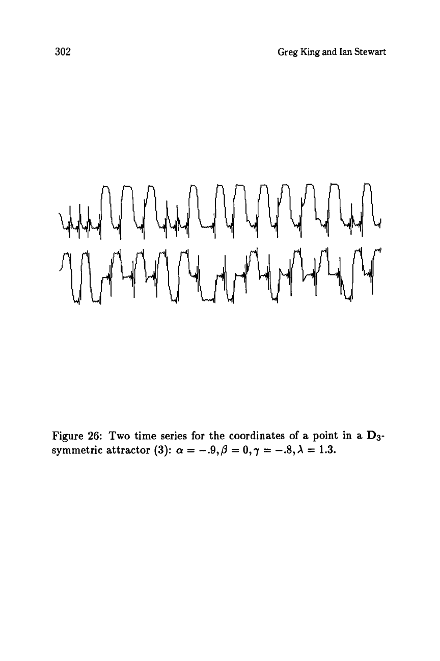
Figure
26:
Two
time series
for
the coordinates
of
a point in a
D3-
symmetric attractor
(3):
a
=
-.9,p
=
O,7
=
-.8,X
=
1.3.
Symmetric Chaos
303
w
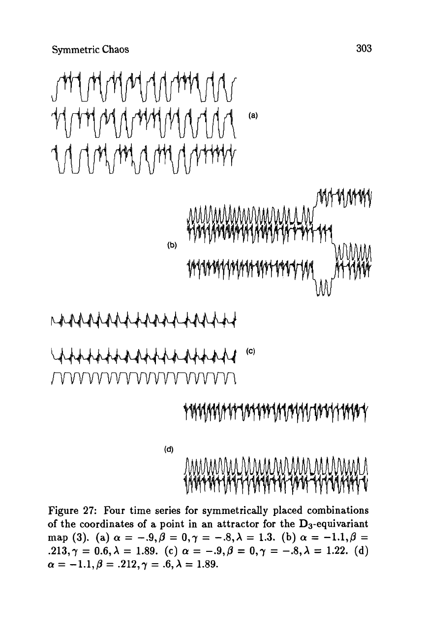
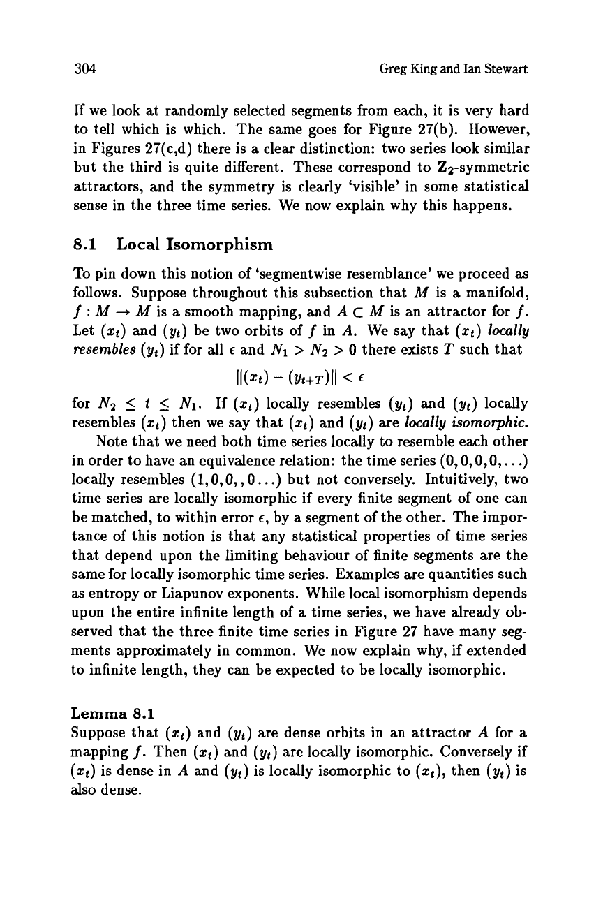
Figure 27: Four time series
for
symmetrically placed combinations
of
the coordinates
of
a point in an attractor
for
the Ds-equivariant
map
(3).
(a)
a
=
-.9,p
=
0,y
=
-.8,X
=
1.3. (b)
a
=
-1.1,p
=
.213,7
=
0.6,
X
=
1.89.
(c)
(Y
=
-.9,p
=
O,7
=
-&A
=
1.22.
(d)
a
=
-1.1,p
=
.2l2,7
=
.6,X
=
1.89.
304
Greg
King
and
Ian
Stewart
If
we look at randomly selected segments from each, it is very hard
to tell which is which. The same goes for Figure 27(b). However,
in Figures 27(c,d) there is
a
clear distinction: two series
look
similar
but the third is quite different. These correspond to Zz-symmetric
attractors, and the symmetry is clearly ‘visible’ in some statistical
sense in the three time series. We now explain why this happens.
8.1
Local
Isomorphism
To pin down this notion of ‘segmentwise resemblance’ we proceed as
follows. Suppose throughout this subsection that
M
is
a
manifold,
f
:
A4
-,
M
is
a
smooth mapping, and
A
c
M
is an attractor for
f.
Let
(zt)
and
(yt)
be two orbits of
f
in
A.
We say that
(zt)
locally
resembles
(yt)
if for all
c
and
N1
>
N2
>
0
there exists
T
such that
ll(4
-
(Yt+T)ll
<
.f
for
N2
5
t
5
N1.
If
(zt)
locally resembles
(yt)
and
(yt)
locally
resembles
(zt)
then we say that
(Q)
and (yt) are
locally
isomorphic.
Note that we need both time series locally to resemble each other
in order to have an equivalence relation: the time series
(0,
0,
O,O,
.
.
.)
locally resembles
(1,0,0,
,
0
..
.)
but not conversely. Intuitively, two
time series are locally isomorphic if every finite segment of one can
be matched, to within error
c,
by
a
segment of the other. The impor-
tance of this notion is that any statistical properties of time series
that depend upon the limiting behaviour of finite segments are the
same for locally isomorphic time series. Examples are quantities such
as
entropy
or
Liapunov exponents. While local isomorphism depends
upon the entire infinite length of
a
time series, we have already ob-
served that the three finite time series in Figure 27 have many seg-
ments approximately in common. We now explain why, if extended
to infinite length, they can be expected to be locally isomorphic.
Lemma
8.1
Suppose that
(zt)
and
(yt)
are dense orbits in an attractor
A
for
a
mapping
f.
Then
(zt)
and
(yt)
are locally isomorphic. Conversely if
(zt)
is dense in
A
and
(yt)
is locally isomorphic to
(q),
then
(yt)
is
also dense.
Symmetric
Chaos
305
Proof
Choose
6
>
0
and consider an arbitrary segment of
(xt)
where
Nz
5
t
I
NI.
Since
(yt)
is dense in
A,
for arbitrary
6
>
0
we can find
k
such that
llyk
-
XN~((
<
6.
By
continuity
of
f,
if we make
6
sufficiently small we then have
)I(x~~+t)
-
(yk+t)ll
<
c
for
all
t
such
that
0
I
t
5
N1
-
m,
which is what we need.
Lemma
8.2
(a) If
A
is compact then
f(A)
=
A.
(b)
If
A
is compact and
(xt)
is
a
dense orbit then for all
k
the orbit
fk(xt)
is dense in
A.
Proof
(a) Since
A
is
an
attractor, it has
a
dense orbit
(xt).
If
y
E
A
then
there exists
a
subsequence
(xtn)
-
y.
If
n
>
0
then
xtn
E
f(A).
So
y
E
f(A).
By compactness
f(A)
is closed,
so
y
E
f(A)
and
f
is onto
as
required.
(b) This now follows since
(fk(xt)
is dense in
fk(A)
=
A.
-
8.2
Equivariant Phase Space Reconstruction
An important technique for the experimental detection of chaos
is
the recognition of deterministic dynamics
-
especially chaos
-
in
an experimental time series.
In
this section we discuss the analogous
problem for equivariant dynamics:
not only must the presence of
deterministic dynamics be detected, but the symmetry of the corre-
sponding attractor must be obtained.
The simplest method, which goes back to Packard
et
al.
[28]
and
Takens
[34],
is to replace the time series
{yt}
by
a
‘moving window’
of length
N,
given by vectors
x;
=
(y;,
. .
.
,
~;+N-I).
Then, for large
enough
N,
generically the attractor formed by the
x;
in
RN
is topo-
logically equivalent to that for the dynamics that gave rise to the
original time series
{yt}.
There is
a
refinement
of
this method, due to Broomhead and
King
[6],
based upon ideas from signal processing. It is formulated for
306
Greg
King
and
Ian
Stewart
signals produced by
a
continuous dynamical system. Broomhead and
King
[7]
explains how to apply these ideas
to
Poincar6 sections, that
is, to mappings, by local analysis. We describe only the technique
as
it applies to continuous dynamical systems.
As
in the Packard-Takens method, we form
a
‘moving window’
of length
N
from this time series, but the difference is that we then
apply principal component analysis to write the resulting vectors in
RN
as
linear combinations of eigenvectors
of
a
correlation matrix.
Intuitively, this process finds the most common patterns among the
vectors in
RN
and expresses each such vector
as
a
linear combination
of such patterns. The dominant patterns, having the largest eigen-
values, are retained: the remainder are considered to be ‘noise’ and
are ignored.
Specifically, define an N-column matrix
X
=
(z;j),
where
1
5
j
5
N
but
i
is arbitrary, by setting
x;,
=
y;+j-1.
Form the
N
x
N
correlation matrix
C
=
X
X
and let its eigenvectors be
~1,
. .
.
,
VN
and corresponding eigenvalues
01,.
.
.
,
UN.
These eigenvalues are
all
real, since
C
is symmetric, and can be arranged in decreasing order:
without loss of generality
01
2
. .
.
2
UN.
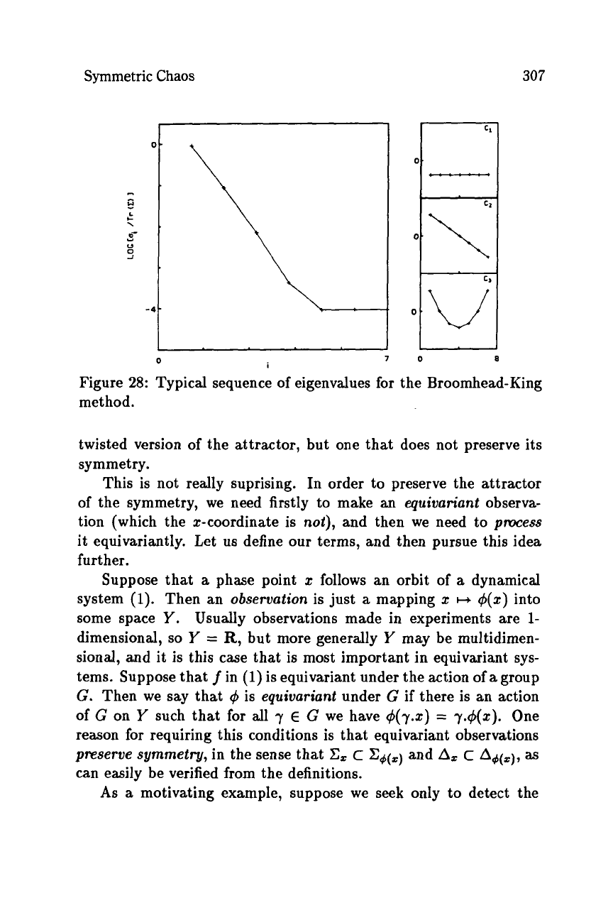
Typically these eigenvalues decrease rapidly and then level
off,
as
in Figure
28.
The point at which they level
off
is the noise
froor
for the observations.
Suppose this starts at
UM+~.
Let
V
=
span(v1,.
.
.
,
VM)
and let the projection of
v
E
RN
into
V
be
ij.
Then
the original time series is replaced by the series of M-dimensional
vectors
fi
where
z;
is the ith row
of
X.
What happens if we apply this method to
a
time series obtained
from an equivariant dynamical system?
As
a
numerical experiment,
we take the
Field-Golubitsky-Chossat
mapping
(3)
with parameters
a
=
l.8,/3
=
O,7
=
1.34164,X
=
-1.8,
which we know produces
the fully symmetric attractor of Figure 4(b). For simplicity we use
the Packard-Takens approach, though similar remarks apply to the
Broomhead-King refinement. We take
N
=
2
(knowing in advance
that the attractor is embedded in
R2),
and let the ‘experimental
measurement’ be the z-coordinate of the point on the attractor. Thus
we plot the pairs (z;,z;+l), for an orbit
(zt,
yt) defining the attractor.
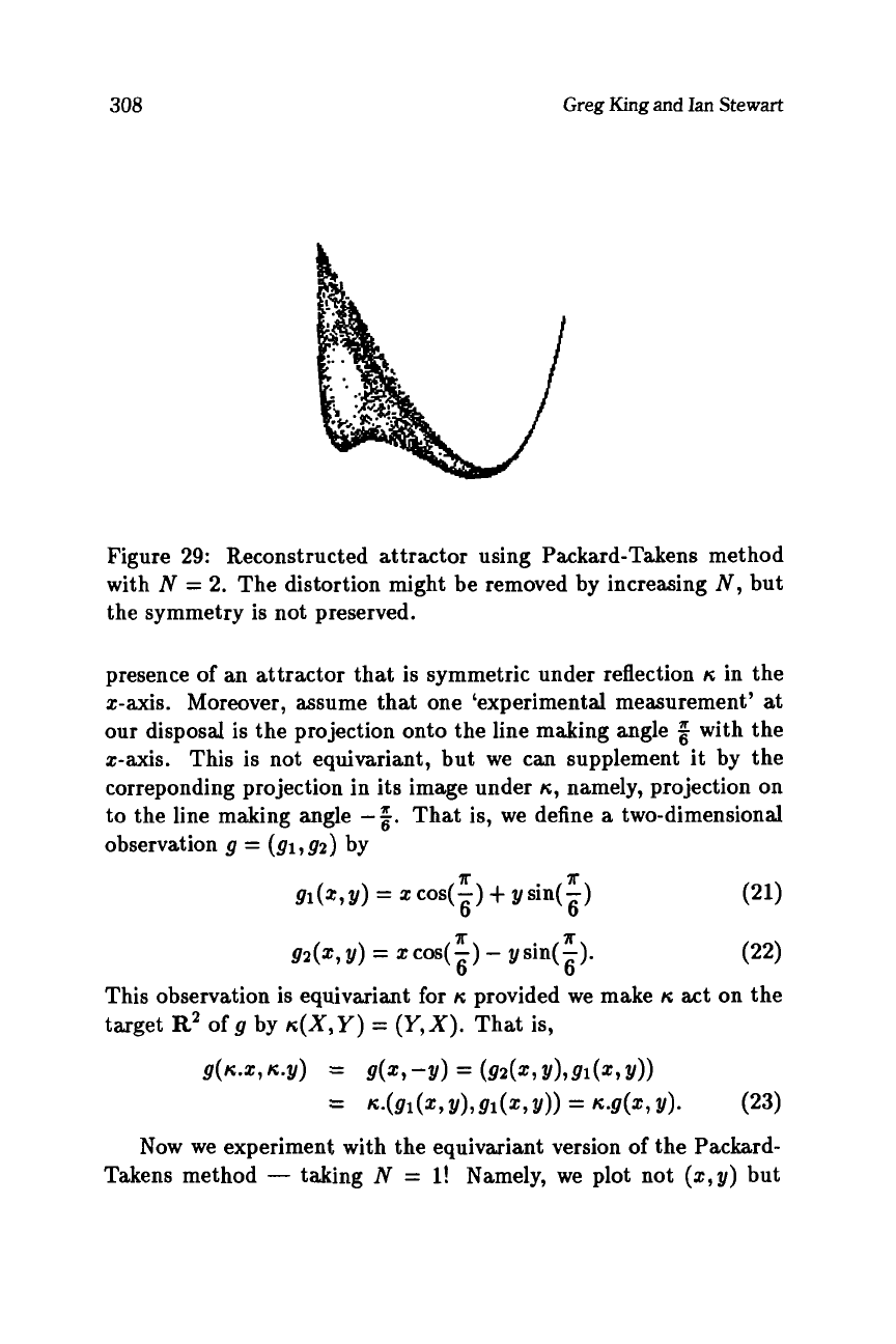
The result is shown in Figure
29.
We can recognise this
as
a
T
Symmetric Chaos
307
0
7
I
0
8
Figure
28:
Typical sequence of eigenvalues for the Broomhead-King
method.
twisted version
of
the attractor, but one that does not preserve its
symmetry.
This
is
not really suprising. In order to preserve the attractor
of the symmetry, we need firstly to make an
equivariant
observa-
tion (which the z-coordinate is
not),
and then we need to
pmess
it equivariantly. Let
us
define
our
terms, and then pursue this idea
further.
Suppose that
a
phase point
z
follows an orbit of
a
dynamical
system
(1).
Then an
observation
is just
a
mapping
z
H
d(z)
into
some space
Y.
Usually observations made in experiments are
1-
dimensional,
so
Y
=
R,
but more generally
Y
may be multidimen-
sional, and it is this case that is most important in equivariant sys-
tems. Suppose that
f
in
(1)
is equivariant under the action of
a
group
G.
Then we say that
4
is
equivariant
under
G
if there is an action
of
G
on
Y
such that for all
7
E
G
we have
d(7.2)
=
y.4(z).
One
reason for requiring this conditions is that equivariant observations
preserve symmetry,
in the sense that
Xz
C
Ed(.)
and
Az
c
Ad(=.,
as
can easily be verified from the definitions.
As
a
motivating example, suppose we
seek
only to detect the
308
Greg
King
and
Ian
Stewart
Figure
29:
Reconstructed attractor using Packard-Takens method
with
N
=
2.
The distortion might be removed by increasing
N,
but
the symmetry is not preserved.
presence
of
an attractor that is symmetric under reflection
K
in the
z-axis.
Moreover, assume that one ‘experimental measurement’ at
our disposal is the projection onto the line making angle with the
z-axis.
This is not equivariant, but we can supplement it by the
correponding projection in its image under
K,
namely, projection
on
to the line making angle
-:.
That is, we define
a
two-dimensional
observation
g
=
(gl
,g2)
by
(22)
A
A
g2(2,y)
=
zcos(-)
-
ysin(-).
This observation is equivariant
for
K
provided we make
K
act on the
target
R2
of
g
by
K(X,Y)
=
(Y,X).
That is,
6 6
Sf(K.2,
K.Y)
=
g(z,
-?I)
=
(g2(z,
Y),gl(z,
?/I>
=
471(z,Y),gl(z,Y))
=
w(z,
Y).
(23)
Now
we experiment with the equivariant version
of
the Packard-
Takens method
-
taking
N
=
l!
Namely, we plot not
(z,y)
but
Symmetric
Chaos
309
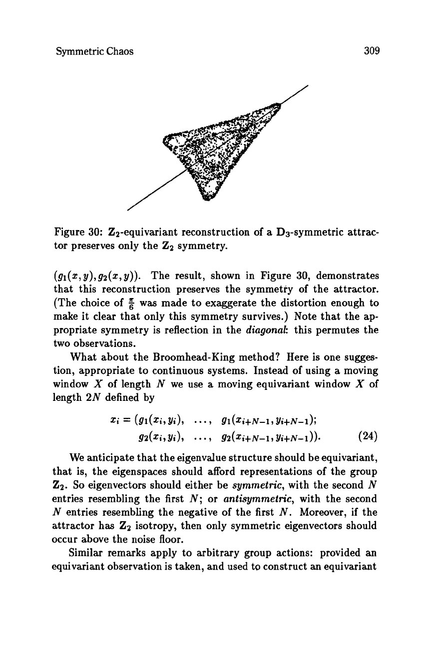
Figure
30:
Zz-equivariant reconstruction
of
a
D3-symmetric attrac-
tor preserves only the Zz symmetry.
(g1(z,
y),gZ(z,
y)).
The result, shown in Figure
30,
demonstrates
that this reconstruction preserves the symmetry of the attractor.
(The choice of was made to exaggerate the distortion enough to
make it clear that only this symmetry survives.) Note that the ap-
propriate symmetry is reflection in the
diagonal:
this permutes the
two observations.
What about the Broomhead-King method? Here is one sugges-
tion, appropriate to continuous systems. Instead
of
using
a
moving
window
X
of
length
N
we
use
a
moving equivariant window
X
of
length
2N
defined by
Xi
=
(gl(zi,yi),
-..
9
gl(zi+N-l,Yi+N-I);
gZ(zi,
yi),
*
*
-
9
gZ(zi+N-l, Yi+N-l)).
(24)
We anticipate that the eigenvalue structure should be equivariant,
that is, the eigenspaces should afford representations of the group
Zz.
So
eigenvectors should either be
symmetric,
with the second
N
entries resembling the first
N;
or
antisymmetric,
with the second
N
entries resembling the negative of the first
N.
Moreover, if the
attractor has
22
isotropy, then only symmetric eigenvectors should
occur above the noise floor.
Similar remarks apply to arbitrary group actions: provided an
equivariant observation is taken, and used to construct an equivariant
