Yangsheng Xu, Yongsheng Ou. Control of Single Wheel Robots
Подождите немного. Документ загружается.

62
3M
od
el-based
Con
trol
β
0
[ ra
d
]
˙
β
0
[ ra
d/s
] ˙α
0
˙γ
0
x
0
[m] y
0
π/3 3 4 -3.660381 1.0 1.0
Table 3.5. Initialparameters in position control.
β
e
[ ra
d
]
˙
β
e
[ ra
d/s
]
x
e
[m] y
e
k
3
k
4
π/2 0 0 0 10 5
Table 3.6. Target and gain parameters in position control.
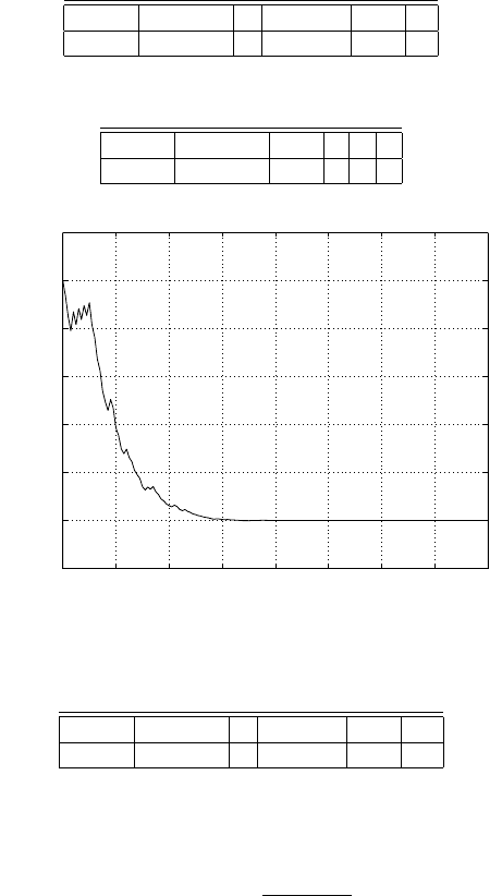
0 2 4 6 8 10 12 14 16
−0.2
0
0.2
0.4
0.6
0.8
1
1.2
Time (s)
x
Fig. 3.24. DisplacementinX.
β
0
[ rad ]
˙
β
0
[ rad/s] ˙α
0
˙γ
0
x
0
[m] y
0
π/2 . 1 0.1 4 -3.660381 0.05 0.05
Table 3.7. Initialparameters in line tracking.
Definition 4 Uanh( . )isaunipolar function described as follows:
Uanh( x )=
1
1+e
− k
7
x
(3.59)
where k
7
is apositive scalarconstant, whichcan be designed. Uanh( . )isshown
as in Figure 3.33.
We substitute Sgn ( . )and Θ ( . )with Tanh( . )and Uanh( . ), respectively.
However, thatthey have different values is aproblem, if x =0.Inareal time
experiment, x =0very seldomappears and cannotbemaintained, because
thereistoo much noise. Thus, it is safe to perform the suggestedsubstitution
fromthis pointofview.
3.3
Con
trolI
mplemen
tation
63
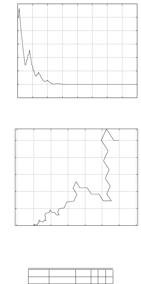
0 2 4 6 8 10 12 14 16
−0.2
0
0.2
0.4
0.6
0.8
1
1.2
Time (s)
y
Fig. 3.25. DisplacementinY.
−0.2 0 0.2 0.4 0.6 0.8 1 1.2
0
0.2
0.4
0.6
0.8
1
X (s)
Y
Fig. 3.26. X-Yoforigin.
β
e
[ rad ]
˙
β
e
[ rad/s] x
e
[m] y
e
k
3
k
5
π/2 0 3 4 10 5
Table 3.8. Target and gain parameters in line tracking.
3.3Control Implementation
An on-board100-MHZ 486 computerwas installed in Gyrovertodeal with
on-board sensing andcontrol. Aflash PCMCIA card is usedasthe com-
64
3M
od
el-based
Con
trol
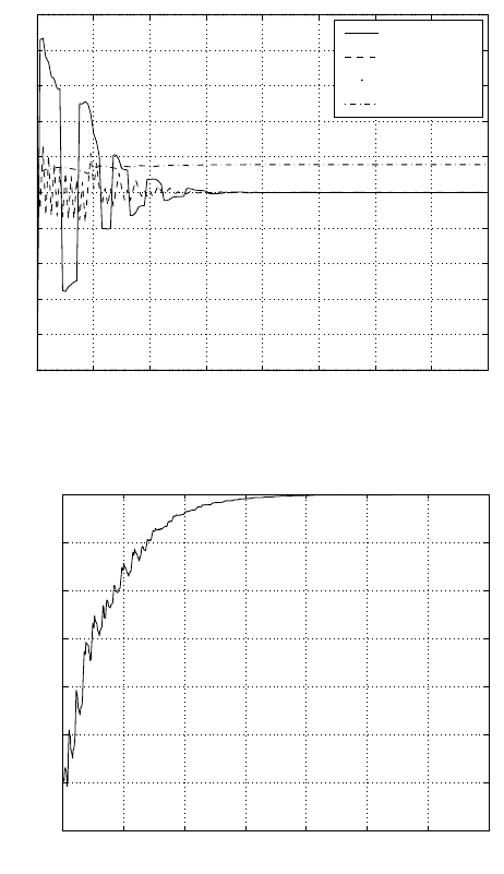
0 2 4 6 8 10 12 14 16
−10
−8
−6
−4
−2
0
2
4
6
8
10
Time (s)
˙γ
˙
β
˙α
β
Fig. 3.27. The joint-space va
riables in po
sition control.
0 5 10 15 20 25 30 35
−0.5
0
0.5
1
1.5
2
2.5
3
Time (s)
x
Fig. 3.28. Line tracking in Xdirection.
puter’s hard diskand communicateswith astationary PC via apair of wireless
modems. Based on this communicationsystem, we can download thesensor
data file fromthe onboardcomputer, send supervising commands to Gyrover,
andmanuallycontrol Gyroverthroughthe stationaryPC. Moreover,aradio
transmitter is installed forahuman operator to remotely control Gyrovervia
thetransmitter’s two joysticks. One operator uses the transmitter to control
the drive speed and tilt angle of Gyrover. Hence,wecan record the operator’s
driving data.
3.3
Con
trolI
mplemen
tation
65
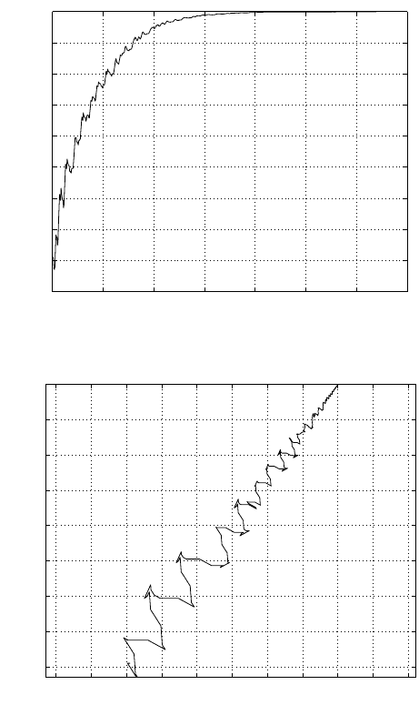
0 5 10 15 20 25 30 35
−0.5
0
0.5
1
1.5
2
2.5
3
3.5
4
Time (s)
y
Fig. 3.29. Line tracking in Yd
irection.
−1 −0.5 0 0.5 1 1.5 2 2.5 3 3.5 4
0
0.5
1
1.5
2
2.5
3
3.5
X (s)
Y
Fig. 3.30. X-Yofinlinetracking.
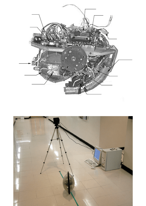
Numerous sensors areinstalled in Gyrovertomeasure state variables(Fig-
ure 3.34).Two pulseencoders areinstalled to measure the spinning rate of the
flywheeland thewheel. Furthermore, we have twogyros andanaccelerometer
to detect the angular velocityofyaw,pitch, roll, and acceleration respectively.
A2-axis tilt sensor has been developedand installed fordirectly measuring
the leanangle andpitchangle of Gyrover. Agyro tilt potentiometer is used
to calculate the tilt angle of theflywheel and its rate change.
Theon-boardcomputerruns on QNX, whichisareal-time micro-kernel
OS developed by QNX Software SystemLimited. Gyrover’s software system
66
3M
od
el-based
Con
trol
0 5 10 15 20 25 30 35
−40
−30
−20
−10
0
10
20
30
40
Time (s)
˙γ
˙
β
˙α
β
Fig. 3.31. The joint-space va
riables in line trac
king.
−5 −4 −3 −2 −1 0 1 2 3 4 5
−1
−0.8
−0.6
−0.4
−0.2
0
0.2
0.4
0.6
0.8
1
X
Y=Tanh(kx)
k=1
k=10
Fig. 3.32. Function Tanh(.).
−5 −4 −3 −2 −1 0 1 2 3 4 5
0
0.1
0.2
0.3
0.4
0.5
0.6
0.7
0.8
0.9
1
X
Y=Uanh(kx)
k=1
k=10
Fig. 3.33. Function Uanh(.).
is dividedi
nt
ot
hree main programs:(1) communication server, (2)
sensor
server, and(3) controller.The communication server is usedtocommunicate
between the on-board computer and astationary personalcomputer(PC)
viaanRS232, whilethe sensorserver is used to handleall the sensors and
actuators. The controller program implementsthe control algorithm andcom-
municatesamong these servers. All programs run independently in order to
allow real-time control of Gyrover. To compensate forthe friction at thejoints,
we adoptthe following approximate mathematical model:
F
f
= µ
v
˙q +[µ
d
+(µ
s
− µ
d
) Γ ] sgn (˙q )(3.60)
where Γ = diag { e
( −| ˙q
i
| /D)
} ,and
3.3
Con
trolI
mplemen
tation
67
Gyro
Accelerometer
Sensors
Assem
bly
Radio Receiver
I/O Board
PowerCable
Tilt Servo
Battery
DriveM
otor and Encoder
Tilt Potentiometer
Speed Controller
Speed Controller
Fig. 3.34. Hardware configuration of Gyrover.
Fig. 3.35. Experiment
in line followingcontrol.
µ
s
∈ R
3 × 3
is the static friction coefficient;
We have µ
v
= diag { 0 . 17, 0 . 15, 0 . 09} , µ
d
= diag { 0 . 1 , 0 . 1 , 0 . 07} , µ
s
=
diag { 0 . 3 , 0 . 25, 0 . 1 } .
µ
v
∈ R
3 × 3
is the viscous friction coefficient;
µ
d
∈ R
3 × 3
is the dynamic friction coefficient;
68
3M
od
el-based
Con
trol
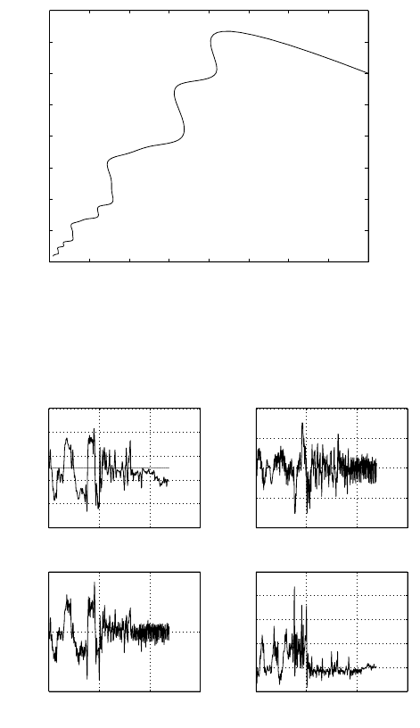
3.3.1Vertical Balance
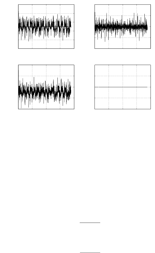
Thepurposeofthis setofexperiments is to keep Gyroverbalanced. Some
experimental resultsare shown in Figure 3.36 andFigure 3.37.
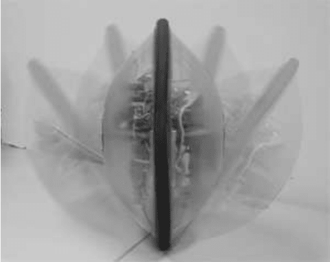
Fig. 3.36. Camera pictures in balance control.
Despite sev
eral successful examples, con
trol laws sometimes ma
yfail.W
e
believeitisbecause the initial condition is set outofthe domain D in Propo-
sition 1. With regard to
balance control,
the initial
condition seems to
be
to
o
narrowfor theconstraint, σ<π/2. If we makeasmall modificationto u
6
as
follows, the controller canbeused in awider range of initial conditions.
u
6
= − ((2 + k
1
)(β − π/2) +(
3+2
k
1
)
˙
β +(2+k
1
)
¨
β + h
1
( t )
˙
β + h
2
( t ) u
5
) /h
3
( t )
where k
1
is ap
ositive
numb
er,whichc
an be
designed.T
op
rove
the subsys-
tem β,
˙
β,
¨
β is asymptotically stabilized, we consider thefollowing Lyapunov
functioncandidate
V
∗
=(β − π/2)
2
/ 2+(
˙
β
+ β − π/2)
2
/ 2+(
¨
β
+(1+k
1
)(
˙
β
+ β − π/2))
2
/ 2 .
Its derivativeis
˙
V
∗
= − ( β − π/2)
2
− k
1
(
˙
β + β − π/2)
2
− (
¨
β +(1+k
1
)(
˙
β + β − π/2))
2
.
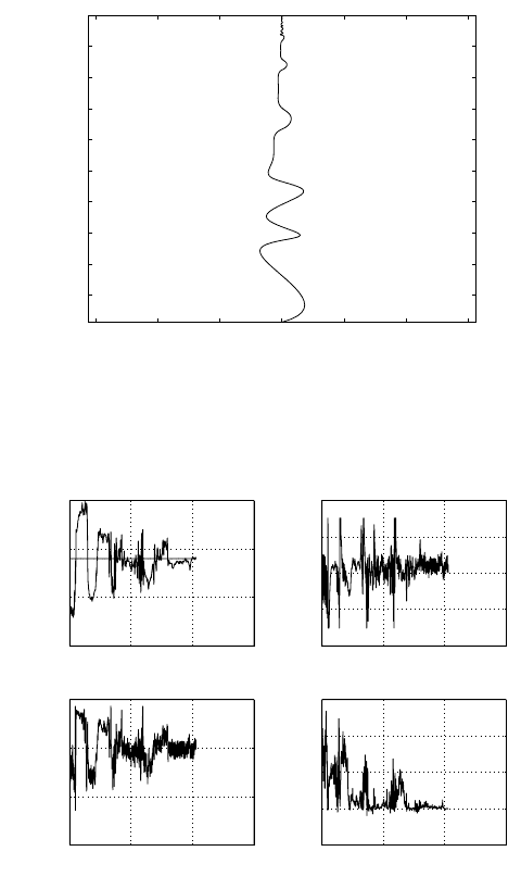
3.3.2 PositionControl
In this experiment, Gyroverisrequired to move fromaCartesian space point
( x
0
,y
0
)tothe originalpoint of Cartesian space, where
x
0
=3mand y
0
=4m.
3.3
Con
trolI
mplemen
tation
69
0 20 40 60 80
40
60
80
100
120
140
Time (s)
β [deg]
0 20 40 60 80
−200
−100
0
100
200
Time (s)
0 20 40 60 80
−40
−20
0
20
40
Time (s)
0 20 40 60 80
−1
−0.5
0
0.5
1
Time (s)
˙
β [deg/sec ]
˙α [deg/sec]
˙γ [deg/sec]
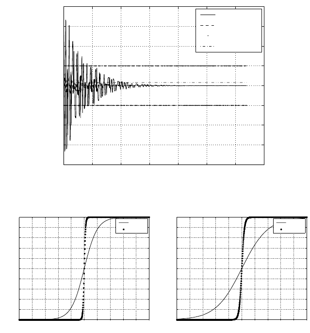
Fig. 3.37. Sensor data in balance control.
We mountahighresolution 2 / 3” ccd, formatCANON COMMUNICATION
CAM
ERA
VC
-C1
on atri
po
d.
Th
ecame
ra ha
sb
een
c al
ib
ra
ted
an
dw
eh
av
e
mapped the field of visiontothe Cartesian space coordinate which is anchored
on theground. The camerahas apixel arrayof768(H ) × 576(V ). In order to
communicate the data, an interface board(
digital I/O) is
installed in
aP
C
andthere arewireless modems to connect the PC andGyrover.
The firstp
roblemexperienced is that the system states exhibited highly
oscillatorybehavior and the second is that control inputs sometimes needed to
switchtoo sharply andfast.Both will cause difficulties forreal time control
andresult in worse performance.Tosolvetheseproblems,wepropose to
replace thesign functions in the controllers with tanh functions.
Let Tanh( . )beabipolar function described as follows:
Tanh( x )=
1 − e
− k
6
x
1+e
− k
6
x
(3.61)
where k
6
is apositive scalarconstant, whichcan be designed.
Let Uanh( . )beaunipolar function described as follows:
Uanh( x )=
1
1+e
− k
7
x
(3.62)
where k
7
is apositive scalarconstant, whichcan be designed.
70
3M
od
el-based
Con
trol
We substitute Sgn ( . )and Θ ( . )with Tanh( . )and Uanh( . ), respectively.
However, thatthey have different values is aproblem, if x =0.Inareal time
experiment, x =0very seldomappearsand cannotbemaintained, because
therei
st
oo
mu
ch
noise.
Th
us,
it
is
sa
fe
to
pe
rform
the
sug
gesteds
ubstitution
fromt
his
po
in
to
fv
iew.
Thetrajectory that Gyrovertraveled is shown in Figure3.38.Anumber
of sensor reading resultsare shown in Figure 3.39.
0 0.5 1 1.5 2 2.5 3 3.5 4
0
0.5
1
1.5
2
2.5
3
3.5
4
•← start
← end
x (m)
y (m)
Fig. 3.38. Trajectories in point-to-pointcontrol.
0 5 10 15
40
60
80
100
120
140
Time (s)
β [deg]
0 5 10 15
−200
−100
0
100
200
Time (s)
0 5 10 15
−50
0
50
Time (s)
0 5 10 15
−20
0
20
40
60
80
Time (s)
˙
β [deg/sec ]
˙α [deg/sec]
˙γ [deg/sec]
Fig. 3.39. Sensor data in point-to-pointcontrol.
3.3
Con
trolI
mplemen
tation
71
3.3.3Path Following
In this experiment, Gyroverisrequired to travelastraight path whichis
ab
out5
ml
ong.
Thet
ra
jectory
th
at
Gy
ro
ve
rt
ra
ve
led
is
sho
wn
in
Figur
e6
.1
1.
An
um
be
ro
fs
ensor
re
adingr
esults
ar
es
ho
w
ni
nF
igure
6.
16.
−3 −2 −1 0 1 2 3
0.5
1
1.5
2
2.5
3
3.5
4
4.5
•← start
← end
x (m)
y (m)
Fig. 3.40. Trajectories in the straightpath test.
0 10 20 30
0
50
100
150
Time (s)
β [deg]
0 10 20 30
−200
−100
0
100
200
Time (s)
0 10 20 30
−100
−50
0
50
Time (s)
0 10 20 30
−50
0
50
100
150
Time (s)
˙
β [deg/sec ]
˙α [deg/sec]
˙γ [deg/sec]
Fig. 3.41. Sensor data in the straightpath test.