Yangsheng Xu, Yongsheng Ou. Control of Single Wheel Robots

Подождите немного. Документ загружается.

4.2

arningb

whereeachofthem is generatedfromanunknown probabilitydistribution

P ( x ,y)containing theunderlying dependency. (Here andbelow, bold face

charactersdenote vectors.)

this

pap

er,

the

term

ill

refer

lassiﬁcation

egression

metho

erms

Supp

ort

ctor

Classiﬁcation(

andS

upp

ort

Vector Regression (SVR) will be usedfor speciﬁcation. In SVR, the basic idea

is to map the data X into ahigh-dimensional feature space F via anonlinear

mapping Φ ,and to do linearregression in this space [108].

f ( x )=(ω · Φ ( x )) + b with Φ : R

→F,ω∈F, (4.16)

where b is athreshold. Thus,linear regression in ahigh dimensional (fea-

ture) space corresponds to nonlinearregression in the lowdimensional input

space R

.Note that thedot productinEquation (4.16)between ω and Φ ( x )

would have to be computedinthis highdimensional space (whichisusually

intractable). If we arenot able to usethe kernel that eventually leavesus

with dot products that can be implicitly expressedinthe lowdimensional

input space R

.Since Φ is ﬁxed,wedetermine ω fromthe data by minimizing

the sum

of the empirical risk

emp

[ f ]and acomplexity term  ω 

,which

enforces ﬂatness in feature space

reg

[ f ]=R

emp

[ f ]+λ  ω 



i =1

C ( f ( x

) − y

)+λ  ω 

, (4.17)

where l denotesthe samplesize ( x

,..., x

), C ( . )isaloss function and λ is a

regularization constant.

Fora

large set of

loss functions, Equation(

4.17) can

be minimized by solving aquadraticprogrammingproblem, which is uniquely

solvable [98]. It

canb

eshown

that thev

ector

ω can be

writteni

erms of the

data po

ints

ω =



i =1

( α

− α

∗

) Φ ( x

) , (4.18)

with α

, α

∗

ing the

solution of the aforementioned quadratic programming

problem [108]. The positiveLagrange multipliers α

and α

∗

arec

alled support

values. They have an intuitiveinterpretation as forces pushingand pulling

the estimate f ( x

)towards the measurements y

[27]. Taking Equation(4.18)

andEquation (4.16)intoaccount, we areable to rewrite the whole problem

in terms of dotproductsinthe lowdimensional input space

f ( x )=



l =1

( α

− α

∗

)(Φ ( x

) · Φ ( x )) + b



l =1

( α

− α

∗

) k ( x

, x )+b.

(4.19)

In Equation(4.19),weintroduce akernel function k ( x

, x

)=Φ ( x

) · Φ ( x

As explained in [15], anysymmetric kernel function k satisfying Mercer’s

conditioncorresponds to adot product in some feature space.

Foramore detailed referenceonthe theory andcomputation of SVM,

readersare referred to [27].

84 4 Learning-based Control

4.2.2 Learning Approach

The skill that we are considering here is the control strategy demonstrated by

a human expert to obtain a certain control target. For example, in controlling a

robotic system, a human expert gives commands by way of a controller, such as

a joystick, and the robot executes the task. The desired trajectory of the robot

given by an expert through a joystick reﬂects the expert’s control strategy. The

goal of the human control strategy learning here is to model the expert control

strategy and according to current states select one command that represents

the most likely human expert strategy. Here, we consider the human expert

actions as the measurable stochastic process and the strategy behind it as the

mapping between the current states and commands. An SVR is employed to

represent human expert strategy for the given task, and the model parameters

are sought through an oﬀ-line learning process. This method allows human

experts to transfer their control strategy to robots. The procedure for SVM-

based control strategy learning can be summarized as follows:

1. Representing the control strategy by an SVM: Choosing a suitable kernel

and structure of an SVM for characterizing the control strategy.

2. Collecting the training data: Obtaining the data representing the control

strategy we want to model.

3. Training the model: Encoding the control strategy into an SVM.

4. Finding the best human performance: Learning/transferring the control

strategy.

For training an SVM learning controller, the system states will usually be

treated as the learning inputs and the control inputs/commands will be the

learning outputs.

Training Example Collection

An SVM does not require a large amount of training samples as do most

ANNs. Scholkopf [23] pointed out that the actual risk R( w ) of the learning

machine is expressed as:

R ( w ) =



 f

( x ) − y  dP ( x ,y) . (4.20)

where P ( x ,y)i

he same distribution deﬁnedi

4.15).T

he problemi

hat

R ( w )isunknown, since

P is unknown.

The straightforwardapproachtominimize the empirical risk,

emp

( w )=



i =1

| f

( x

) − y

 ,

turns outnot to guaranteeasmall actualrisk R ( w ), if the number l of training

examples is limited. In other words: asmall error in the trainingset does

4.2

arningb

not necessarily imply ahigh generalization ability(i.e., asmall error on an

independenttest set). This phenomenon is often referred to as overfitting.To

solvethe problem, novelstatisticaltechniques have been developedduring the

last

ars.

learning

problem,

the

cture

nimiza

tion

(SRM)p

rinciplei

asedo

fact

thatf

w ∈ Λ and l>

ith

probabilityofatleast 1-η ,the bound

R ( w ) ≤ R

emp

( w )+Φ (

log ( η )

)(4.21)

holds,where the confidence termΦis deﬁned as

Φ (

( η )



h ( log

2 l

+1) − log ( η/4)

The parameter h is called the VC ( Vapnik- Chervonenkis)dimension of a

set of functions, whichdescribes the capacityofaset of functions. Usually,to

decrease the R

emp

( w )t

ome bound, most ANNs with complex mathematical

structure have averyhigh value of h .Itisnotedthatwhen n/h is small (for

example less

than 20,the trainings

ample is

small in size),

Φ hasal

arge

value. When this occurs, performance poorly represents R ( w )with R

emp

( w ).

As ar

esult, according to

the

SRM principle, alarge trainings

ample size is

requiredtoacquireasatisfactorylearningmachine.However, by mapping the

inputs in

afeature space usingar

elatively simple mathematical function,

suchasap

olynomial kernel,anSVM hasas

mall va

lue for

h ,a

nd at thes

ame

time maintainsthe R

emp

( w )inthe same bound. To decrease R ( w )with Φ ,

therefore, requires small

n ,w

hichisenoughalso for small

h .

Trainingprocess

The ﬁrstproblem, before beginning training,istochoose between SVR or

SVC; the choiceb

eing dependentonspecial control

systems. Fo

xample, our

experimentalsystem Gyrover hasthe control commands U

and U

.Their

values are scaled to the tilt angle of theﬂywheel and the driving speed of

Gyrover respectively.Thus, forthis case,wewill choose SVR.However, for

mart wheelchair system, forinstance,the con

trol commands1,2,3a

nd 4

correspond to “goahead”, “turnleft”, “turnright”,and “stop” respectively.

Sincethis is aclassiﬁcationproblem, it is better to choose SVC.

Thesecond problem is to select akernel. Thereare severalkindsofkernel

appropriate foranSVM [27]. The main function of kernelsinanSVM is to

map the input space to ahigh dimensional feature space,and at that space the

feature elements have alinear relationwith the learning output. In most cases,

it is diﬃcult to set up this kind of linear relations. This is because usually we

do notknowthe mathematicalrelationbetween the input and output. Thus,

it is better to test more kernelsand choose the best one.

86 4 Learning-based Control

The third problem is about “scaling”. Here, scaling refers to putting each

Column’s data into a range between − 1 and 1. It is important to void the

outputs if they are seriously aﬀected by some states, for the “unit’s” sake.

Moreover, if some states are more important than others, we may enlarge

their range to emphasize their eﬀect.

Time Consideration

An SVM usually requires more time in obtaining the optimal weight matrix for

the same set of training samples than a general neural network learner, such

as Exappropriation neural networks (BPNN). An SVM determines the weight

matrix through an optimization seeking process, whereas an ANN determines

it by modifying the weights matrix backward from the diﬀerences between the

actual outputs and estimated outputs. [15] and Vapnik [108] show how t raining

an SVM for the pattern recognition problem (for a regression problem it is

similar but a l ittle more complex) leads to the following quadratic optimization

problem (QP)OP1.

( OP1)minimize : W ( α )=−



i =1



i =1



j =1

k ( x

, x

)(4.22)

subject to :



i =1

=0 ∀ i :0≤ α

≤ C (4.23)

Thenumberoftraining examples is denoted by l . α is avector of l variables,

wheree

achc

omponent

corresponds to at

raining example (

). C is

theboundary of α

.The solutionofOP1 is the vector ˆα forwhich(4.22) is

minimized and the

constraints

(4.23)are fulﬁlled. Deﬁning the matrix

Q as

(

Q )

= y

k ( x

), this can be

equivalently writtena

minimize : W ( α )=− α

1 +

Q α (4.24)

subject to : α

y =0 , 0 ≤ α ≤ C 1 (4.25)

Sincethe size of thematrix

Q is l

,the size of theoptimization problem

depends on thenumberoftraining examples.However, most general ANNs,

(suchasBPNN)havelinear relationship with the sample size. Because of this,

SVMs usuallyneed more trainingtime than most other ANNs. Moreover, if

thesize of thesample is large, this phenomenonismuchmoreserious. For

example, for asize of 400example set, an SVMneeds about10minutes to

complete thetraining process andaBPNN requiresabout 1minutewill ﬁnish.

If the size of thesample reaches 10, 000, an SVM willneed more than 100hours

to complete, whereas, theBPNN just requiresabout 25 minutes.

4.2 Learning by SVM 87

Learning Precise Consideration

In practice applications, the control process of an SVM learner is much

smoother than general ANN learners. The reason for this is that many ANNs

and HMM methods exhibit the local minima problem, whereas for an SVM the

quadratic property guarantees the optimization functions are convex. Thus it

must be the global minima.

Moreover, for the class of dynamically stable, statically unstable robots

such as Gyrover, high learning precision is required and very important. This

is because the learning controller will be returned to control the robot and

form a new dynamic system. Larger errors in control inputs will cause sys-

tem instability and control process failure. During our experiments, we always

required several training sessions to produce a successful general ANN con-

troller. However, after training the SVM learning controller it always worked

well immediately.

4.2.3 Convergence Analysis

Here, we provide the convergence analysis of the learning controller, but not

the learning convergence of SVMs. From the practice point of view, we con-

sider the local asymptotical convergence instead of global or semi-global con-

vergence. This is because, in the training process, we can only collect data

in a region of systems variables, called the “working space”. It is a set of all

the points that the system states can reach. Furthermore, we deﬁne “region

of operation” D as a meaningful working region, a subset of “working space”.

Usually, region of operation D is a compact subset of the full space R

with its

origin. Thus, with these local data, we almost can not obtain a highly precise

training result in the full space R

In fact, for this class of learning controller, it can only drive the system

to converge into a bounded small neighborhood of the origin (or desirable

equilibrium). This is because of the SVM model learning error. For a local

asymptotical convergence, the region of attraction is a critical issue. The re-

gion of attraction may not be larger or equal to “region of operation” D , but

should be desirable large.

Problem Statement

x = f ( x, u ) , (4.26)

where

x ∈ R

system states

u ∈ R

( m ≤ n )control inputs

˙x time derivatives of thestates x

f ( · ):R

n + m

→ R

unknown nonlinearfunction

88 4 Learning-based Control

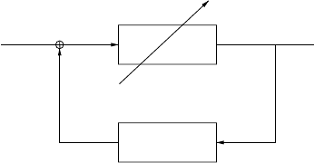
x(0)

u(t)

x(t)

Plant

Human Control

Fig. 4.6. Thepractical system and the human control from adynamic system.

Thecontrol objective can be describedas: ﬁndacontinuous control law u =

u ( x ), suchthatall of the states of the abovesystem (4.26) asymptotically

tendtoabounded small neighborhood of theorigin.

Assume that apractical system hasbeen well controlled by ahuman ex-

rt andt

he all states of

thesystem have

been putintoina

small neighbor-

hood

of origin. Thepractical system andt

he hu

man controlformad

ynamic

system shown in Figure4.6. Usually,acontinuous-time control process is

approximately considereda

sap

rocess of

fast discrete-time sampling. This

continuous-time nonlinear controlsystem is approximately described by the

diﬀerence equation of

theform

x ( t +1)=f

( x ( t ) , u

( t )) (4.27)

where x =[x

,..., x

]

∈ R

is the state

vector,

∈ R

is the human

control vector, f

=[f

,..., f

]

: R

n + m

→ R

is aset of unknown nonlin-

ear functions. We

assume throughout the paperthatthe state vector

x of the

system can be measured.

There is alearningcontroller forthe dynamicsystem (4.27), whichisob-

tainedb

yoﬀ-line learning fromad

ata table pro

duced by

the human expert

demonstration, shown in Figure4.7. The diﬀerence Equation(4.28) approxi-

mately described the learningcontroller











ˆx

( t +1)=

( x ( t ) , u ( t )) = f

( x ( t ) , u ( t )) + e

( x ( t ) , u ( t ))

ˆx

( t +1)=

( x ( t ) , u ( t )) = f

( x ( t ) , u ( t )) + e

( x ( t ) , u ( t ))

ˆx

( t +1)=

( x ( t ) , u ( t )) = f

( x ( t ) , u ( t )) + e

( x ( t ) , u ( t ))

( t +1)=f

n +1

( x ( t ) , u ( t ))

( t +1)=f

n + m

( x ( t ) , u ( t )),

(4.28)

where

x =[ˆx

, ˆx

,..., ˆx

]

∈ R

is the estimation forthe state vector x

and

,...,

]

: R

n + m

→ R

is an estimationfor f

. e =

[ e

,...e

]

= f

−

is amodel error.

u =[u

,..., u

]

∈ R

is the

4.2

arningb

estimationfor thehuman control vector u

and f

=[f

n +1

n +2

,..., f

n + m

]

n + m

→ R

is the estimation fornext time human control.

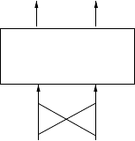
Neural networks

x(t)

u(t)

x(t+1) u(t+1)

Fig. 4.7. Alearning controller.

If we use thelearningcontroller u to control the system, we have a

new closed-form contin

uous-time dynamicsystem and it

approximately de-

scribed

thediﬀerence equationo

he form



x ( t +1)=f

( x ( t ) , u ( t ))

u ( t +1)=f

( x ( t ) , u ( t )).

(4.29)

Furthermore, we let X =[x

]

and f =[f

]

,the

X ( t +1)=f ( X ( t )) (4.30)

and let

X =[

]

and

f =[

]

,the

X ( t +1)=

f (

X ( t )) (4.31)

where (4.31) is an estimation for (4.30).

The aim of this section is twofold: to formulate conditions for the system

(4.30) to be stable and to determine the domain of attraction, if it is stable.

Lyapunov Theory

A very important tool in the stability analysis of discrete dynamic systems is

given by Lyapunov’s theory [65], [61].

Deﬁnition 1: A function V ( X ) is said to be positive deﬁnite in a region W

containing the origin if (i) V (0) = 0. (ii) V [ X ( t )] > 0 for all x ∈W, X = 0.

Deﬁnition 2: Let W be any set in R

containing the origin and V : R

→

R . We say that V is a Lyapunov function of Equation (4.30) on W if (i) V is

continuous on R

. (ii) V is positive deﬁnite with respect to the origin in W .

(iii) ∆V ( t ) ≡ V [ X ( t + 1)] − V [ X ( t )] ≤ 0 along the trajectory of (4.30) for all

X ∈W.

90 4 Learning-based Control

The existance of a Lyapunov function assures stability as given by the

following theorem.

Theorem 1: If V is a Lyapunov function of (4.30) in some neighborhood

of an equilibrium state X = 0, then X = 0 is a stable equilibrium.

If in addition − ∆V is positive deﬁnite with respect to X = 0, then the

origin is asymptotically stable.

So far, the deﬁnition of stability and asymptotical stability are in terms

of perturbations of initial conditions. If the model error e is small, one hopes

that at least qualitatively, the behavior of the original system and that of the

perturbed one will be similar. For the exact relation, stable under perturba-

tionsneeds to be deﬁned [94].

Deﬁnition 3: Let X ( X

, t ) denote the solution of (4.30) with the initial

condition X

= X ( X

, 0). The origin X = 0 is said to be stable under pertur-

bations if for all  > 0 there exists δ

(  ) and δ

(  ) such that ||X

|| < δ

and

||e ( t, X ) || < δ

for all k > 0 imply X ( X

, t ) <  for all t ≤ 0.

If in addition, for all  there is an r and a T (  ) such that ||X

|| < r and

||e ( t, X ) || < δ

(  ) for all t > 0 imply ||X ( X

, t ) || <  for all t > T (  ), the

origin is said to be strongly stable under perturbations(SSUP).

Strongly stable under perturbations (SSUP) means that the equilibrium is

stable, and that states started in B

⊂ Ω actually converge to the error bound

at limited time. Ω is called a domain of attraction of the solution (while the

domain of attraction refers to the largest such region, i.e., to the set of all

points such that trajectories initialed at these points eventually converge to

the error bound.

With this in mind the following theorem [61], [94] can be stated:

Theorem 2: If f is Lipschitz continuous in a neighborhood of the equilib-

rium, then the system (4.30) is strongly stable under perturbations iﬀ it is

asymptotically stable.

In this paper, Support Vector Machine (SVM) will be considered as a

neural network structure to learn the human expert control process. In the

next section, a rough introduction to the SVM learner that we will use, will

be provided.

Convergence Analysis

There are many kernels that satisfy the Mercer’s condition as described in

[27]. In this paper, we take a simple polynomial kernel in Equation (4.19):

K ( X

, X ) = ((X

· X ) + 1)

, (4.32)

where d is user deﬁned (Taken from [108]).

After the oﬀ-line training process, we obtain the support values ( α and

∗

) and the corresponding support vectors. Let X

be sample data of X .

By expanding Equation (4.19) according to Equation (4.32), Let

f ( X )=

4.2

arningb

[

,...

m + n

]

be avector.

is anonhomogeneousformofdegree d in

X ∈ R

n + m

(containing allmonomials of degree ≤ d )



0 ≤ k

+ k

+ ...+ k

n + m

≤ d

...x

n +1

...u

n + m

, (4.33)

where k

,..., k

n + m

arenonnegative integers, and c

∈ R areweighting

coeﬃcients. j can be 1 , 2 ,..., M ,where M =(

n + m + d

n + m

). Then,

f ( X )=C + A



X + g ( X ) , (4.34)

where C =[c

..c

m + n

]

onstan

ector,



∈ R

( n + m ) × ( m + n )

eﬃcientmatrix forthe degree 1in X and g ( X )=[g

( X ) ,g

( X ) ,...g

n + m

( X )]

is avector. g

( X )isamultinomial of degree ≥ 2of X .

Assume that we hadbuilt m + n number of multiple-input-one-output

SVM models. Accordingto[108], SVM can approximate to amodel in any

accuracy,i

he training data nu

er is large enough,

i.e. forany

>0, if ¯

is the sample data number and e is the modelerror, there exists a N>0,

suchthatif¯n>N, e<.The following assumptions aremadefor theSVM

models.

Assumption1: Fo

rsystem (4.30), in

the

region

D ,the

samp

data is largeenough.

Remark 3.1:

Assumption 1i

sually required in control

design with

neural

networks forfunctionapproximation [31],[53]. Then fromthe aboveanalysis,

we have assumption2.

Assumption 2: Fo

rsystem (4.30), in

the

region

D ,t

he learning precision

is high.

Hence, if the mo

del(4.31) is suﬃcient

ly accurate, accordingt

oEquation

(4.34), the system (4.30) can be transformed to theEquation(4.35)

X ( t +1)=C + A



X + g ( X ) , (4.35)

Sincethe originisanequilibriumpoint of thesystem, we have C =

[0, 0 ,...0]

andt

hen

X ( t +1)=A



X + g ( X ) , (4.36)

Thus, we can use thefollowing theorem to judgethe system (4.30) is strongly

stable under perturbations(SSUP) or not.

Theorem3: Forthe system (4.30), with assumptions 1and 2being satisﬁed

in the region D ,if − A =(I − A



)isapositivedeﬁnite matrix and

I is a

( n + m ) × ( n + m )identical matrix, then theclosed-form system (4.30) is

strongly stable under perturbations(SSUP).

Proof: Let V = X

X .Then, V is positivedeﬁnite. By diﬀerentiating V

alongthe trajectoriesof X onegets

∆V =

∂V

∂X

∆X =2X∆X. (4.37)

92 4 Learning-based Control

Substituting (4.36) and (4.37) into it, then

∆V = 2 X ( A



− I ) X + 2 Xg( X ) = 2 XAX + 2 Xg( X ) .

If we let µ be the smallest eigenvalue of the matrix − A , then we have µ | z |

≤

( − A ) z, ∀ z . The properties of g ( X ) imply the existence of a function

ρ ( X ) such that lim

X → 0

ρ ( X ) = 0 and | g ( X ) |≤ρ ( X ) | X | . We can then get the

estimate

∆V = 2 XAX + 2 Xg( X ) ≤−| X |

( µ − 2 ρ ( X )).

The fact that ρ tends to zero as X tends to zero implies the existence of a

constant r > 0 such that ρ ( X ) < µ/2 whenever | X |≤r . It follows that − ∆V

is positive deﬁnite in | X | < r and the system (4.30) is asymptotically stable.

Moreover, since f is Lipschitz continuous and according to Theorem 2, we

know that the system is strongly stable under perturbations (SSUP).

Remark 3.2: The technique used in the proof can in principle give an ap-

proach in estimating the domain of attraction Ω . This value of r will however

often be quite conservative. The arrangement of this is a critical property to

evaluate the practical value of the SVM learning controller. In the next part

of this section, we will provide a better and more practical method to estimate

the domain of attraction Ω .

Computation of Stability Region

The problem of determining stability regions (Subsets of domain of attrac-

tion) or robust global stability [106], of nonlinear dynamical systems is of

fundamental importance in control engineering and control theory.

Let ∆X( t ) = X ( t + 1) − X ( t ), we transform the system (4.36) to

∆X = AX + g ( X ) , (4.38)

where we assumed that A is a negative deﬁnite matrix, i.e., all eigenvalues of A

have strictly negative real parts. Thus, the problem in this part is to estimate

the domain of attraction of X = 0. The main tool in achieving this goal is the

use of an appropriate Lyapunov function. In fact, there are almost an inﬁnite

kind of Lyapunov functions that can be applied for this aim. However, a large

number of experiments show that the type of quadratic Lyapunov functions,

which are chosen, usually can work out a desirable stability region if an SVM

learning controller has ﬁne performance in practical control experiments. In

the following we will address the quadratic Lyapunov function.

V ( X ) = X

PX, (4.39)

where P is a positive deﬁnite symmetric ( n + m ) × ( n + m ) matrix. Assuming

that the matrix

Q = − ( A

P + PA) , (4.40)