Wong H.-S.P., Akinwande D. Carbon Nanotube and Graphene Device Physics

Подождите немного. Документ загружается.

3.1 Introduction 49

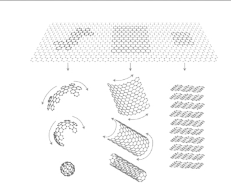
Fig. 3.3 Two-dimensional graphene can be considered the building block of several carbon

allotropes in all dimensions, including zero-dimensional buckyballs, 1D nanotubes, and

3D graphite. Reprinted by permission from Macmillan Publishers Ltd (A. K. Geim and

K. S. Novoselov, Nat. Mater., 6, (2007) 183–91, copyright (2007)).

graphene into a sphere produces buckyballs, folding into a cylinder produces nan-

otubes, and stacking several sheets of graphene leads to graphite. Furthermore,

cutting graphene into a small ribbon results in nanoribbons, which are the sub-

ject of contemporary research. As a result, understanding the electronic properties

of graphene is of central importance in explaining, for example, the electronic

properties of carbon nanotubes and nanoribbons.

In graphene, the 2s orbital interacts with the 2p

and 2p

orbitals to form three

hybrid orbitals with the electron arrangement shown in Figure 3.1b. The sp

interactions result in three bonds called σ -bonds, which are the strongest type

of covalent bond. The σ -bonds have the electrons localized along the plane con-

necting carbon atoms and are responsible for the great strength and mechanical

properties of graphene and CNTs. The 2p

electrons forms covalent bonds called

π-bonds, where the electron cloud is distributed normal to the plane connecting

carbon atoms. The 2p

electrons are weakly bound to the nuclei and, hence, are

relatively delocalized. These delocalized electrons are the ones responsible for the

electronic properties of graphene and CNTs and as such will occupy much of our

attention.

50 Chapter 3 Graphene

3.2 The direct lattice

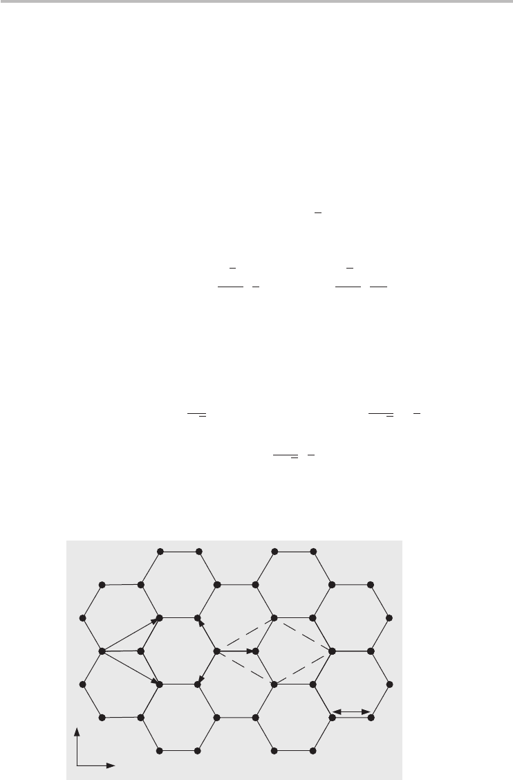
Graphene has a honeycomb lattice shown in Figure 3.4 using a ball-and-stick

model. The balls represent carbon atoms and the sticks symbolize the σ -bonds

between atoms. The carbon–carbon bond length is approximately a

C−C

≈ 1.42 Å.

The honeycomb lattice can be characterized as a Bravais lattice with a basis of

two atoms, indicated as A and B in Figure 3.4, and these contribute a total of two

π electrons per unit cell to the electronic properties of graphene. The underlying

Bravais lattice is a hexagonal lattice and the primitive unit cell can be considered

an equilateral parallelogram with side a =

√

C−C

= 2.46 Å. The primitive unit

vectors as deﬁned in Figure 3.4 are



√



, a



√

−2



, (3.1)

with |a

|=|a

|=a. Each carbon atom is bonded to its three nearest neighbors

and the vectors describing the separation between a type A atom and the nearest

neighbor type B atoms as shown in Figure 3.4 are



√



, R

=−a

+ R



−

√

, −



=−a

+ R



−

√



, (3.2)

with |R

|=|R

|=a

C−C

c–c

Fig. 3.4 The honeycomb lattice of graphene. The primitive unit cell is the equilateral

parallelogram (dashed lines) with a basis of two atoms denoted as A and B.

3.3 The reciprocal lattice 51

3.3 The reciprocal lattice

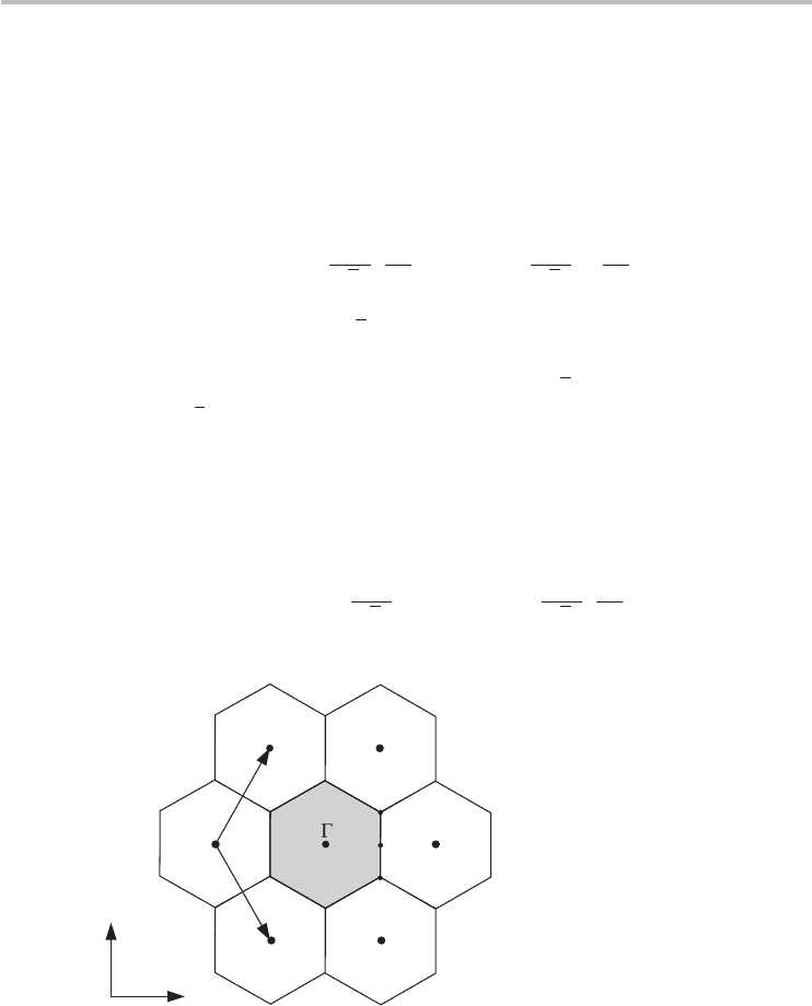
The reciprocal lattice of graphene shown in Figure 3.5 is also a hexagonal lattice,

but rotated 90

◦

with respect to the direct lattice. The reciprocal lattice vectors are

(from Eq. (2.34))



2π

√

2π



, b



2π

√

, −

2π



, (3.3)

with |b

|=|b

|=4π/

√

3a. The Brillouin zone, which is a central idea in

describing the electronic bands of solids, is illustrated as the shaded hexagon

in Figure 3.5 with sides of length b

=|b

√

3 = 4π/3a and area equal

to 8π

√

. There are three key locations of high symmetry in the Brillouin

zone which are useful to memorize in discussing the dispersion of graphene. In

Figure 3.5, these locations are identiﬁed by convention as the -point, the M-point,

and the K-point.

The -point is at the center of the Brillouin zone, and the vectors

describing the location of the other points with respect to the zone center are

M =



2π

√



, K =



2π

√

2π



, (3.4)

Fig. 3.5 The reciprocal lattice of graphene. The ﬁrst Brillouin zone is the shaded hexagon with the

high symmetry points labeled as , M, and K located at the center, midpoint of the side,

and corner of the hexagon respectively. The K



-point, which is also an hexagonal corner

(adjacent to the K-point), is essentially equivalent to the K-point for most purposes.

The naming of the high-symmetry points for every Bravais lattice has its origins in group theory;

for reference, see M. S. Dresselhaus, G. Dresselhaus and A. Jorio, Group Theory: Application to

the Physics of Condensed Matter (Springer, 2008).

Sometimes a distinction is made between the K-point and K



-point, particularly in the discussion of

intervalley or interband electron scattering by lattice vibrations (more about this in Chapter 7). For

our current studies, we will simply call out the K-points to refer to all the corners of the hexagonal

Brillouin zone unless explicitly stated otherwise.

52 Chapter 3 Graphene

with |M |=2π/

√

3a, |K|=4π/3a, and |M K|=2π/3a. There are six

K-points

and six M-points within the Brillouin zone.

The unique solutions for the energy bands of crystalline solids are found within

the Brillouin zone and sometimes the dispersion is graphed along the high-

symmetry directions as a matter of practical convenience. Furthermore, we shall

sometimes use the terminology k-space to refer to the reciprocal lattice and the

vector that locates any point within the Brillouin zone is the wavevector k. That is,

every allowed point (also synonymous with the term allowed state when referring

to the dispersion) within the Brillouin zone can be reached by k.

3.4 Electronic band structure

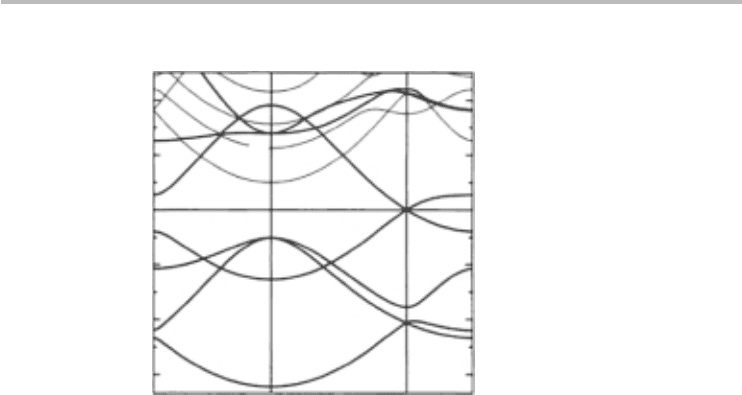
The band structure of graphene is shown in Figure 3.6. This band structure was

computed numerically from ﬁrst principles and shows many energy branches

resulting from all the π and σ electrons that form the outermost electrons

of carbon. Our purpose here is to develop an analytical description of the

band structure that would nurture our intuition for the device physics and lead

to simple algebraic expressions for the relevant device and material parame-

ters. Invariably, developing an analytical expression for the band structure of a

solid generally requires solving the time-independent Schrödinger’s equation in

3D space:

H (k, r) = E(k)(k, r), (3.5)

where H is the Hamiltonian operator that operates on the wavefunction  to

produce the allowed energies E. The Hamiltonian for an independent electron in

a periodic solid is given by

H =



∇

+ 

U (r − R

), (3.6)

where the former term in the Hamiltonian is the kinetic energy operator and the

latter term is the potential energy operator. R

is the ith Bravais lattice vector, N is

the number of primitive unit cells, and U (r−R

) is the potential energycontribution

from the atom centered in the ith primitive unit cell. The potential energy is the

sum of the single-atom potentials and, hence, is periodic and Coulombic in nature

(1/r dependence). Substituting the Hamiltonian into the Schrödinger equation

results in a second-order partial differential equation. In practice, constructing a

wavefunction that satisﬁes the partial differential equation is non-trivial, requiring

deep thought, and may consist of iterating over several trial wavefunctions until

a suitable wavefunction is determined. In any case, acceptable wavefunctions in

a crystalline solid must satisfy Bloch’s theorem, which proves that valid traveling

3.4 Electronic band structure 53

–6

–12

–18

⌫

Wave vector

Energy (eV)

Fig. 3.6 The ab-initio band structure of graphene, including the σ and π bands. The Fermi energy

is set to 0 eV. Adapted with permission from M. Machón et al., Phys. Rev. B, 66, (2002)

155410. Copyright (2002) by the American Physical Society.

waves in a lattice have the property

(r + R) = e

ik·R

(r), (3.7)

where R is a Bravais lattice vector. In addition, periodic boundary conditions are

imposed on the wavefunctions to determine the allowed values of the wavevector

that leads to running waves:

(r) = (r + S) = e

ik·S

(r), ⇒∴ e

ik·S

= 1, (3.8)

where S is the size vector whose lengths in all the coordinates of space are the

spatial dimensions of the lattice.

In general there are two limiting techniques for obtaining a satisfactory wave-

function and associated band structure.

In one limiting case, called the nearly-free

electron model, the outermost valence electrons are essentially considered free

except for a weak Coulomb attraction to their respective nucleus. As a result, the

Both techniques (nearly-free electron and tight-binding models) were developed by Felix Bloch

during his Ph.D. research in the late 1920s. Bloch was very ﬂuent in Fourier transforms and his

application of Fourier analysis to electrons in solids gave him original insights into their properties.

Bloch later went on to become the ﬁrst Nobel laureate at Stanford University in 1952.

54 Chapter 3 Graphene

full periodic potential is replaced by a weak perturbing potential and Schrödinger’s

equation is solved by employing standard perturbation techniques in quantum

mechanics. This model yields solutions in terms of modulated plane waves

( ∼ u(r)e

ik·r

), and the associated energy bands often have a parabolic struc-

ture. This model has been shown to be useful in describing the band structure of

some metals.

The other limiting technique, called the tight-binding model, inherently assumes

that the outermost electrons are to a large extent localized (i.e. tightly bound) to

their respective atomic cores and, hence, described by their atomic orbitals with

discrete energy levels. However, because the atoms are not isolated but exist in

an ordered solid, the orbitals of identical electrons in neighboring atoms in a

solid with N unit cells will overlap, with the major consequence that the N dis-

crete energy levels will inevitably broaden into quasi-continuous energy bands

with N states/band owing to Pauli’s exclusion principle. The overlap of wave-

functions by and large renders inaccurate the use of atomic orbitals in describing

electrons in a solid. Nonetheless, for the special case of a very small overlap,

one might still be able to use the tight-binding model to obtain an approximate

analytical band structure that we hope will be in good agreement with experi-

mental measurements or more sophisticated numerical ab-initio band structure

computations.

We have to choose between these two models in order to develop an analyt-

ical electronic band structure. For the particular case of graphene, a variety of

arguments can be proposed (mostly based on experience, because band structure

calculation is as much an art as it is science) to support the choice of a particular

model. Fortunately, we know from chemistry that graphene can be considered a

large carbon molecule and, as such, a ﬁrst guess might be to employ standard quan-

tum chemistry techniques such as linear combination of atomic orbitals (which we

have been calling tight binding) for deriving molecular band structures. Further-

more, visual inspection of the ab-initio computations (Figure 3.6), particularly

around the Fermi energy (E

, the energy at 0 eV),

shows a linear dispersion,

suggesting that perhaps a nearly-free electron model might not be our ﬁrst choice,

since that would require a large number of plane waves. If the dispersion had

been parabolic-like, a nearly-free electron model might arguably be a more attrac-

tive initial choice. Accordingly, we chose the tight-binding model. How well the

tight-binding model agrees with ab-initio computations or experimental data is the

ultimate judge of whether the chosen model is indeed useful. We will now proceed

to dive into the detailed mathematics and derive the tight-binding band structure

of graphene.

The most mobile electrons are at the Fermi energy. We will use E

= 0 eV casually for now until

later, at the end of this section, when a formal deﬁnition is presented to identify its location in the

band structure of graphene.

3.5 Tight-binding energy dispersion 55

3.5 Tight-binding energy dispersion

Rather than discussing very broadly the tight-binding formalism, we will focus on

the speciﬁc problem of calculating the band structure of graphene. The primary

challenge in the tight-binding model is to construct a suitable wavefunction that

satisﬁes Bloch’s theorem while retaining the atomic character. From this wave-

function, the subsequent calculation of the energy bands is fairly straightforward,

though it can be mathematically tedious. Fortunately, a general tight-binding

ansatz

for the wavefunction has been constructed previously in terms of lin-

ear combinations of atomic orbitals originally proposed by Bloch in 1928. For

graphene, which has a basis of two, the tight-binding wavefunction is a weighted

sum of the two sub-lattice Bloch functions:

(k, r) = C



(k, r) + C



(k, r), (3.9)

where the subscripts A and B denote the two different atoms in the graphene unit

cell (see Figure 3.4). The weights (C

, C

) are, in general, functions of k but

independent of r. For a crystal with a basis of m, the sum will include m sub-lattice

terms. The ansatz expresses the Bloch functions as a linear combination of the

atomic orbitals or wavefunctions which are assumed to be known:



(k, r) =

√



ik·R

φ(r − R

) (3.10)



(B, r) =

√



ik·R

φ(r − R

), (3.11)

where N is the number of unit cells in the lattice and R

) are the Bravais

lattice vectors identifying the locations of all type A (B) atoms in the graphene

lattice. The atomic orbitals φ belong to a class of functions known as Wannier

functions, which are orthonormal functions that are sufﬁciently localized such that,

at distances increasingly removed from the center point R

, the functions decay

to zero very rapidly. The sum is over all the lattice vectors, and 1/

√

N serves as

normalization constant for the Bloch functions in the strict limit when the Wannier

function in cell j has zero overlap with neighboring Wannier functions.

Ansatz is a German word for an educated guess whose validity is based on the accuracy of its

predictions. Observe that the wavefunction is not computed directly from solving Schrödinger’s

equation, but simply postulated as meeting basic requirements such as Bloch’s theorem. Use of an

ansatz is a common technique in quantum physics to describe constructions of solutions to

non-trivial differential equations.

The Bloch functions are not exact wavefunctions because they are not normalized when we include

some ﬁnite overlap. However, they are the best tight-binding ansatz we have that is not overly

complicated and is still suitable for analysis with useful accuracy.

56 Chapter 3 Graphene

The Bloch functions must satisfy Bloch’s theorem stated in Eq. (3.7):



(r + R



) =

√



ik·R

k · R

φ(r + R



− R

)



(r + R



) =

ik·R

√



ik·(R

−R



)

φ(r − (R

− R



)). (3.12)

The differencebetween two Bravais lattice vectorsis another Bravais lattice vector;

therefore:



(r + R



) =

k·R



√



ik·R

φ(r − R

) = e

ik·R





(r). (3.13)

Additionally, the Bloch functions must satisfy the periodic boundary conditions

stated in Eq. (3.8). Let us express the reciprocal lattice variable k in terms of its

coordinate components, k = k

x + k

y, and let the size vector of the graphene

Bravais lattice be S = aNox + aNoy, where No =

√

N . Imposing the periodic

boundary conditions

ik·S

= cos[ak

No + ak

No]+i sin[ak

No + ak

No]=1, (3.14)

which is only satisﬁed when

2πp

aNo

, k

2πp

aNo

, p = 0, 1, 2, ...,No− 1, (3.15)

where the allowed set of wavevectors that yield unique solutions for the energy

dispersion are limited to the ﬁrst Brillouin zone. The maximum number of k-states

in the Brillouin zone is No

= N , which can hold 2N electrons, where the factor

of 2 is due to spin degeneracy.

With the formalities out of the way, we can now proceed to solve for the

energy bands of graphene. Inserting Eq. (3.9) into the Schrödinger equation we

obtain

H 

(k, r) + C

H 

(k, r) = E(k)C



(k, r) + E(k)C



(k, r). (3.16)

Multiplying by the complex conjugate of 

, and separately by the complex

conjugate of 

, generates two separate equations:



∗

H 

+ C



∗

H 

= EC



∗



+ EC



∗



∗

H 

+ C



∗

H 

= EC



∗



+ EC



∗



(3.17)

As a refresher, mathematics is very precisely formulated in quantum mechanics, including the

order of multiplication, because the operations may not be commutative.

3.5 Tight-binding energy dispersion 57

where we have dropped the dependence on k and r for convenience. Integrat-

ing both equations over the entire space occupied by the lattice (denoted by )

produces







∗

H 

dr + C







∗

H 

dr = EC







∗



dr + EC







∗









∗

H 

dr + C







∗

H 

dr = EC







∗



dr + EC







∗



dr.

(3.18)

It is customary to employ the following symbolic deﬁnitions to make the equations

more manageable:







∗

H 

dr, S







∗



dr, (3.19)

where H

are the matrix elements of the Hamiltonian or transfer integral and have

the units of energy. S

are the overlap matrix elements betweenBloch functions and

are unitless. We can simplify the matrix elements by observing that, since the two

atoms in the unit cell are identical, therefore, the overlap between all type-Aatoms

must be the same as the overlap between all type-B atoms; that is, S

= S

and H

= H

. In addition, H

and S

correspond to physical observables and

hence are Hermitian, which leads to the condition H

= H

∗

and S

= S

∗

Then:

− ES

) = C

(ES

− H

) (3.20)

∗

− ES

∗

) = C

(ES

− H

). (3.21)

Our primary interest here is to obtain an expression for the energy bands. This

system of two linear equations can be solved easily by the method of substitution.

Solving for C

in Eq. (3.21) and substituting into Eq. (3.20) yields a quadratic

equation, which is readily solved for the energy:

E(k)

=−

(k) +



(k)

− 4(S

(k)

−|S

(k)|

)(H

(k)

−|H

(k)|

)

2(S

(k)

−|S

(k)|

)

(3.22)

It is worthwhile remembering that the integration of pairs of a conjugated wavefunction is what

has real probabilistic meaning.

58 Chapter 3 Graphene

with

(k) = (2H

(k)S

(k) −S

(k)H

∗

(k) −H

(k)S

∗

(k)). (3.23)

The positive and negative energy branches in Eq. (3.22) are called the conduction

(π

∗

) and valence (π) bands respectively,

and will be deﬁned to correspond to

positive and negative energy values in a while. Up till now we have not fully

explored tight binding in the mathematical development of the energy bands.

To make further progress in Eq. (3.22), we will now make explicit use of the

assumptions belonging to the tight-binding formalism.Additionally, since our goal

is to develop an analytical equation for the band structure that will resemble the ab-

initio computation in Figure 3.6 (particularly around the Fermi energy), insightful

visual observations of Figure 3.6 will be brought to bear on the problem at hand in

order to arrive at a ﬁnal solution for the energy bands of graphene. The assumptions

and related mathematical consequences are:

1. Nearest neighbor tight-binding (NNTB) model: The wavefunction of an electron

in any primitive unit cell only overlaps with the wavefunctions of its near-

est neighbors. This is easily understood by means of Figure 3.4. The nearest

neighbors of a type-A atom in the graphene lattice are three equivalent type-B

atoms. NNTB stipulates that the p

wavefunction of a type-A atom overlaps

with the p

wavefunctions of its three nearest neighbors, and zero overlap with

wavefunctions from farther atoms. Mathematically, this simpliﬁes Eq. (3.22)

considerably, as the Hamiltonian matrix element reduces to

(k) =







∗

H 

dr =



−ik·R

ik·R





∗

(r − R

)H φ(r − R

)dr (3.24)



ik·(R

−R

)

= E

, (3.25)

where δ

is the Kronecker delta function. The constant term E

is nominally

close to the energy of the 2p orbital in isolated carbon, but not exactly the same

because the Hamiltonian of the lattice (Eq. (3.6)) has a periodic potential, in

contrast to the single Columbic potential of the isolated atom. Similarly, the

The π and π

∗

are the preferred terminology in chemistry, used to describe bonding and

anti-bonding interactions (or energies) respectively. The anti-bonding interactions are higher in

energy than the bonding interactions.