Wong H.-S.P., Akinwande D. Carbon Nanotube and Graphene Device Physics

4.3 The CNT lattice 79

0 1 2 3 4 5 6 7 8 9 10 11 12 13 14 15

16 17 18 19 20 21 22 23 24 25 26 27 28 29 30 31 32

(30,0)

(45,0)

(15,0)

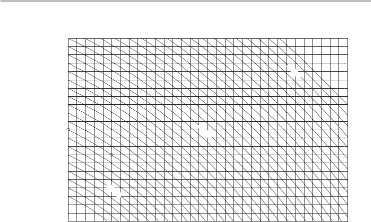
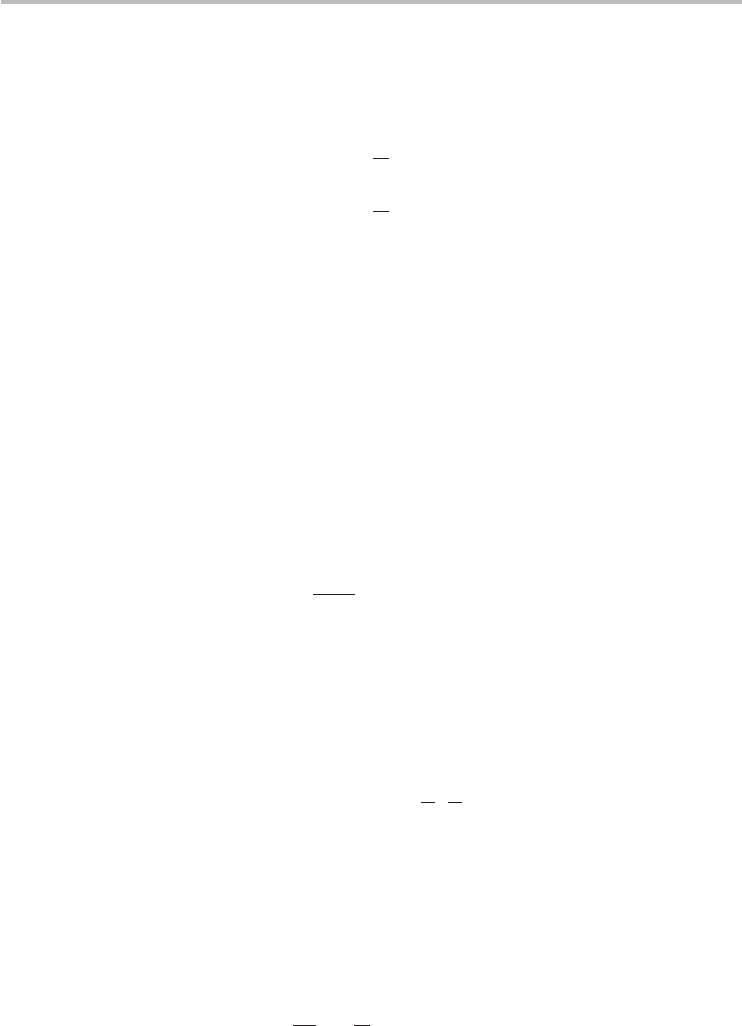
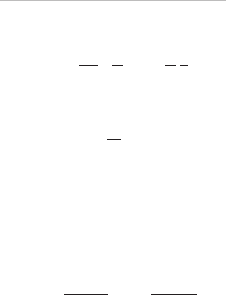
Fig. 4.5 Constant-diameter contour plot of Eq. (4.4). The contour lines represent the constant

diameter of an (n, 0) CNT, and some contour lines have been labeled with their

corresponding (n, 0) index for convenience. As an example, the circles show that a (19, 0)

CNT has identical diameter to a (16, 5) nanotube.

lattice, unique values of the chiral angle are restricted to 0 ≤ θ ≤ 30

◦

. For the

particular exercise of Figure 4.4, θ = 30

◦

. In general, all armchair nanotubes have

a chiral angle of 30

◦

, and θ = 0

◦

for all zigzag nanotubes.

In order to determine the primitive unit cell of the CNT, we need to consider

the translation vector which deﬁnes the periodicity of the lattice along the tubular

axis. Geometrically, T is the smallest graphene lattice vector perpendicular to

. As can be seen from Figure 4.4, T = (1, −1) for all armchair nanotubes.

Similarly, the translation vector for all zigzag nanotubes can be visually deduced

to be T = (1, −2). More broadly, the translation vector can be computed from

the orthogonality condition C

· T = 0. Let T = t

+ t

, where t

and t

are

integers. Therefore:

· T = t

(2n + m) + t

(2m + n) = 0. (4.6)

Determining the acceptable solution for t

and t

requires a subtle interplay involv-

ing mathematical analysis and visual insight. There are two orthogonal directions

(±90

◦

) relating T to C

, and solving for either direction leads to an equivalent

solution for the translation vector. Let us restrict the direction to +90

◦

as shown in

Figure 4.4a. Then, according to the orientation deﬁnition of the lattice vectors a

and a

, t

must be a positive integer and t

must be a negative integer for T to be

80 Chapter 4 Carbon nanotubes

+90

◦

with respect to C

. With this visual insight, one set of integers that satisfy Eq.

(4.6)is(t

, t

) = (2m +n, −2n −m). However, deeper thinking reveals that there

are several sets of integers that are alsosolutions ofEq. (4.6). For instance, consider

an (8, 2) CNT; (t

, t

) = (12, −18) is a solution, but so are (t

, t

) = (12, −18)/2,

, t

) = (12, −18)/3, and (t

, t

) = (12, −18)/6. The actual acceptable solution

that leads to the shortest translation vector is (t

, t

) = (12, −18)/6 = (2, −3),

where the factor of 6 is the greatest common divisor of 12 and 18. Hence, the

acceptable solution for Eq. (4.6)is

T = (t

, t

) =



2m + n

, −

2n + m



, (4.7)

where g

is the greatest common divisor of 2m +n and 2n +m. The length of the

translation vector is

|T |=T =

√

3|C

√

3πd

. (4.8)

The chiral and translation vectors deﬁne the primitive unit cell of the CNT,

which is a cylinder with diameter d

and length T . Some auxiliary results that are

useful to compute include the surface area of the CNT unit cell, the number of

hexagons per unit cell, and the number of carbon atoms per unit cell. The surface

area of the CNT primitive unit cell is the area of the rectangle deﬁned by the C

and T vectors, | C

× T|. The number of hexagons per unit cell N is the surface

area divided by the area of one hexagon:

N =

× T |

× a

2(n

+ nm + m

)

2|C

. (4.9)

This simpliﬁes to N = 2n for both armchair and zigzag nanotubes. Since there are

two carbon atoms per hexagon, there are a total of 2N carbon atoms in each CNT

unit cell. A summary of the geometric parameters and associated equations for

CNTs nanotubes are listed in Table 4.1. Speciﬁc values of the geometric param-

eters for selected nanotubes ranging in diameter from 1 to 3 nm are shown in

Table 4.2.

In order to gain hands-on familiarity with the conceptual construction of a CNT,

the reader is encouraged to construct a nanotube from the blank graphene sheet in

Figure 4.14 at the end of this chapter. As an example, the reader can construct a

(4, 1) CNTand conveniently verify it with the construction shownin Figure 4.6. For

the full construction experience, the reader should physically fold the coincident

points in the lattice onto each other to create a paper model of the CNT.

4.4 CNT Brillouin zone 81

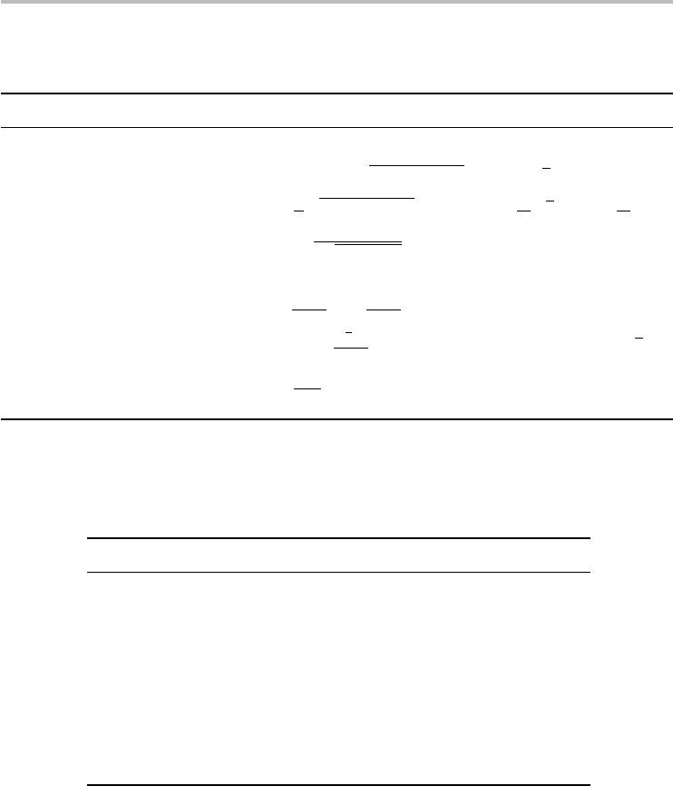
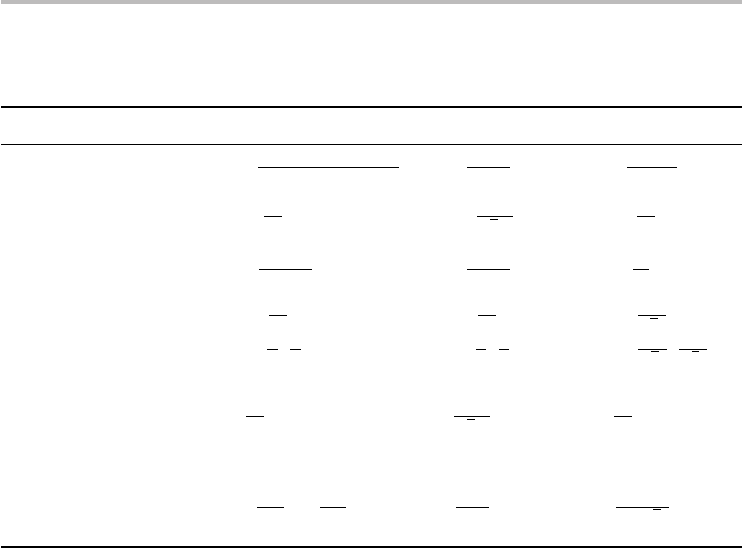
Table 4.1. Table of parameters and associated equations for CNTs.

Symbol Name cCNT aCNT zCNT

chiral vector C

= na

+ ma

= (n, m) C

= (n,0)

length of chiral vector C

=|C

|=a



+ nm + m

= a

√

3nC

= an

diameter d



+ nm + m

√

3 d

θ chiral angle cos θ =

2n+m

√

+nm+m

θ = 30

◦

θ = 0

◦

greatest common divisor g

≡ gcd(2m + n,2n + m) g

= 3ng

= n

T translation vector T =

2m+n

−

2n+m

T = a

− a

T = a

− 2a

T length of translation vector T =

√

T = aT= a

√

N number of hexagons/cell N =

N = 2nN= 2n

The primitive basis vectors a

and a

are deﬁned according to Eq. (4.1). cCNT stands for chiral CNT, aCNT

for armchair CNT, and zCNT for zigzag CNT.

Table 4.2. Table of speciﬁc values for selected CNTs of diameters ∼1–3 nm.

(nm) C

(nm) T (nm)  (deg) NE

(eV)

(10, 4) 0.98 3.07 0.89 16.1 52 0

(10, 5) 1.04 3.25 1.13 19.1 70 0.86

(13, 0) 1.02 3.20 0.43 0 26 0.84

(15, 15) 2.03 6.40 0.25 30 30 0

(16, 5) 1.49 4.67 8.10 13.2 722 0.60

(16, 14) 2.04 6.40 5.54 27.8 676 0.43

(19, 0) 1.49 4.67 0.43 0 38 0.58

(26, 0) 2.04 6.40 0.43 0 52 0.44

(32, 0) 2.51 7.87 0.43 0 64 0.35

(38, 0) 2.98 9.35 0.43 0 76 0.30

The bandgap E

is computed from the tight-binding band structure of CNTs,

which is discussed in Sections 4.6 and 4.8.

4.4 CNT Brillouin zone

Given the primitive unit cell of CNTs developed in the previous section, we are

now in a position to construct the CNT reciprocal lattice and Brillouin zone which

will subsequently aid us in determining its electronic band structure. The focus

will mostly be on the ﬁrst Brillouin zone, which contains the unique values of the

allowed wavevectors and energies. In a way analogous to the path taken in the

prior section to construct the CNT physical structure from the honeycomb lattice

of graphene, we will discover that the Brillouin zone of CNTs is composed of a

82 Chapter 4 Carbon nanotubes

(4,1)

(2 -3)

(a) (b)

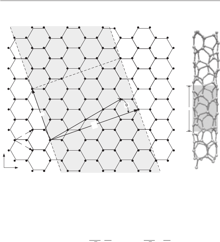
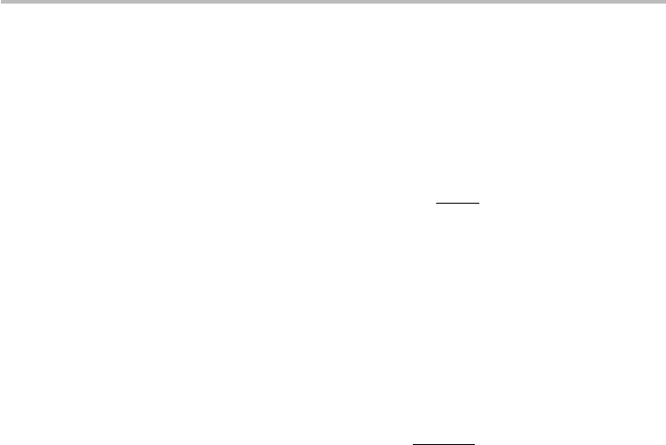
Fig. 4.6 Construction of a chiral CNT. (a) A (4, 1) CNT is constructed from the lattice of graphene.

Points A, B, C, and D are used in a similar manner as in Figure 4.4. (b) Cylindrical

structure of the (4, 1) CNT.

series of cross-sections or line cuts of the reciprocal lattice of graphene. The basis

vectors for graphene’s reciprocal lattice are



2π

√

2π



, b



2π

√

, −

2π



. (4.10)

The wavevectors deﬁning the CNT of the ﬁrst Brillouin zone are the reciprocals

of the primitive unit cell vectors given by the reciprocity condition previously

discussedinChapter 2(Eq.(2.34)):

i(K

)·(C

+T)

= 1, (4.11)

where K

is the reciprocal lattice vector along the nanotube axis and K

is along

the circumferential direction, both given in terms of the reciprocal lattice basis

vectors of graphene (b

, b

). Equation (4.11) simpliﬁes to

· K

= 2π, T · K

= 0, (4.12)

· K

= 0, T · K

= 2π. (4.13)

4.4 CNT Brillouin zone 83

Employing the expressions for C

, T, and N in Table 4.1, the wavevectors can be

derived algebraically:

(mb

− nb

), (4.14)

(−t

+ t

). (4.15)

The lengths of the reciprocal lattice wavevectors are inversely proportional to the

CNT lattice dimensions, i.e. |K

| =2π /T and |K

|=2π/C

. K

and K

in a sense

describe the nanotube Brillouin zone.

The next step is to determine the allowed wavevectors within the Brillouin

zone that lead to Bloch wave functions. Let us consider a nanotube of length

= N

T where N

is the number of CNT unit cells in the nanotube. The

allowed wavevectors k along the axial direction are obtained from the periodic

boundary conditions on the Bloch wave functions:

ψ(0) = ψ(L

) = e

ikN

ψ(N

T ), ⇒∴ e

ikN

= 1, (4.16)

resulting in the set of wavevectors

k =

2π

l, l = 0, 1, ..., N

− 1, (4.17)

where the maximum integer value of l is determined from the requirement that

unique solutions for k are restricted to the ﬁrst Brillouin zone, i.e. maximum

(k)<|K

|=2π/T .

In the limit where the CNT is very long, for instance L

 T

or N

 1,

then the spacing between k-values vanishes and, to ﬁrst-order, k can

be considered a continuous variable along the axial direction:

k =



−



, (4.18)

where the wavevector has been re-centered to be symmetric about zero consistent

with standard Brillouin zone convention.

Applying the same periodic boundary conditions to determine the allowed

wavevectors q along the circumferential direction yields

ψ(0) = ψ(C

) = e

iqC

ψ(0), ⇒∴ e

iqC

= 1, (4.19)

q =

2π

j =

j = j|K

|, j = 0, 1, ..., j

max

. (4.20)

Recall from Chapter 2 that unique values for k and energy are always contained within the ﬁrst

Brillouin zone. Any k-value outside the ﬁrst Brillouin zone can be mathematically translated back

into the ﬁrst Brillouin zone by a reciprocal lattice vector.

This requirement is often satisﬁed by practical CNTs. Furthermore, theoretical work has shown

that a continuously varying k remains a fairly reasonable approximation for CNTs as short as

10 nm. See A. Rochefort, D. R. Salahub and P. Avouris, Effects of ﬁnite length on the electronic

structure of carbon nanotubes. J. Phys. Chem. B, 103, (1999) 641–6.

84 Chapter 4 Carbon nanotubes

123

450

(a) (b)

2 /a

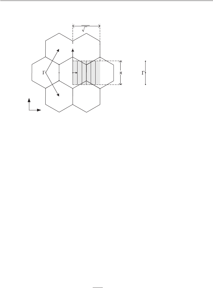
Fig. 4.7 Brillouin zone of a (3, 3) armchair CNT (shaded rectangle) overlaid on the reciprocal

lattice of graphene. The numbers refer to j = 0, 1, ..., 5 for a total of N = 6 1D bands in

the CNT Brillouin zone. The central hexagon is the ﬁrst Brillouin zone of graphene, and

the high-symmetry points (, M, and K) of graphene’s Brillouin zone are also indicated.

The area of the CNT Brillouin zone is equal to the area of graphene’s Brillouin zone. (b)

The high-symmetry points of a line representing a CNT 1D band is illustrated.

We observe that the q-values are separated by a gap that is much greater than the

spacing in k-values, i.e. 2π/C

 2π/L

for long CNTs with lengths L

 C

Therefore, the q variable is quantized or discretely spaced compared with the

relatively continuous k variable, which implies that the allowed CNT wavevectors

in the Brillouin zone are composed of a series of lines as shown in Figure 4.7a.

These lines are basically 1D cuts of graphene’s reciprocal lattice. The ﬁnal question

we have to resolve to obtain the complete set of 1D lines is the maximum value

of j in Eq. (4.20) that yields the total set of unique values for q. To answer this

question we deduce that since the unique wavevectors are discrete set of line cuts of

graphene’sreciprocal lattice, then any two line cuts or q-valuesthat are separated by

a reciprocal lattice vector of graphene must be equivalent. The shortest reciprocal

lattice vector of graphene that is an integer multiple K

is N K

As a result, the

maximum value of q is less than N |K

|, and hence

q =

2π

j, j = 0, 1, ..., N − 1. (4.21)

We noted in Chapter 3 that the K



-point is essentially equivalent to the K-point except under certain

inquiries. A case in point is during conservation of momentum in interband electron scattering in

CNTs(moreaboutthisinChapter7).

given by Eq. (4.15) is a CNT reciprocal lattice vector but not a graphene reciprocal lattice

vector. To obtain a reciprocal lattice vector that is common to both CNT and graphene requires

multiplying K

by N, NK

=−t

+ t

4.4 CNT Brillouin zone 85

(a)

(b)

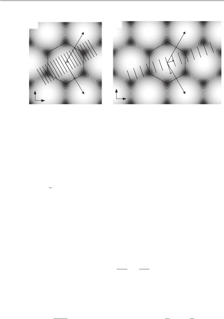
Fig. 4.8

Brillouin zone of (a) (10, 0) CNT and (b) a (4, 1) CNT, overlaid on the contour plot of the

conduction band of graphene (darker shades corresponds to lower energies). The Brillouin

zone of CNTs consists of the series of dark lines representing the N (20 and 14

respectively) 1D bands. The Brillouin zone of graphene is the hexagon. Note that the N

lines have been folded to be symmetric with graphene’s hexagonal Brillouin zone for

convenience (the unfolded lines only exist in the +K

direction). The lengths of the lines

are |K

|=2π/T .

Figure 4.8 shows the Brillouin zones for the (10, 0) and (4, 1) CNTs. The area of

the Brillouin zone of a nanotube is equal to the area of graphene’s Brillouin zone

(8π

√

), which is a consequence of the fact that CNT 1D wavevectors are

cuts of graphene’s 2D Brillouin zone. Table 4.3 is a summary of the expressions

for the reciprocal lattice vectors and wavevectors deﬁned in this section.

We now strive to combine expressions for the allowed axial and circumferen-

tial Brillouin zone wavevectors (Eqs. (4.18) and (4.21) respectively) in order to

generate an expression for any arbitrary allowed state or wavevector within the

Brillouin zone. This general Brillouin zone wavevector k is what will be used to

compute the allowed energies in the band structure of CNTs and is given by

k = k

+ q

, (4.22)

where K

/|K

| and K

/| K

| are the unit vectors in the axial and circumferential

directions respectively. Substituting for |K

|, |K

|, and q from Table 4.3 yields

k = k

2π/T

+ jK



j = 0, 1, ..., N − 1, and −

< k <



. (4.23)

In summary, each value of j corresponds to a line or 1D band with wave vectors k

ranging from −π/T to +π/T . This is one of the most important results the reader

should appreciate.

86 Chapter 4 Carbon nanotubes

Table 4.3. Summary of CNT reciprocal lattice vectors and Brillouin zone wavevectors.

Symbol Name cCNT aCNT zCNT

circumferential

lattice vector

(m+2n)b

+(n+2m)b

2(n

+nm+m

)

| length of K



2π



2π

√

3an

2π

axial lattice

vector

−b

K =−

| length of K

2π

√

k axial Brillouin

zone

wavevector

k =



−



k =



−



k =



−

√



q circumferential

Brillouin

zone

wavevector

q =

2π

jq=

2π

√

3an

jq=

2π

k Brillouin zone

wavevector

k = k

+ q

k =

2π/a

+ jK

k =

2π/

√

+ jK

The primitive basis vectors b

and b

are deﬁned according to Eq. (4.10). j is an integer from 0 to N − 1.

4.5 General observations from the Brillouin zone

In the previous section we learned that the ﬁnite width C

of CNTs leads to quan-

tization of the CNT Brillouin zone, which essentially results in the CNT Brillouin

zone being composed of a series of 1D cuts of the reciprocal lattice of graphene.

This implies that the CNT band structure will be 1D cross-sections of the band

structure of graphene. Before actually computing the CNT band structure, we can

arrive at very important broad conclusions from insights gained from leveraging

our understanding of the electronic structure of graphene.

Let us consider an armchair and zigzag CNTto get our intuition running, and then

generalizetoachiralnanotube.WerecallfromChapter2thattheconductionand

valence bands of graphene touch at the K-points, where the highest equilibrium

occupied states (corresponding to the Fermi energy) exist. The degeneracy or

touching of the bands at a K-point resulted in the absence of a bandgap which

explains the metallic behavior of graphene. At every other point in the Brillouin

zone of graphene there exists an energy gap between the conduction and valence

bands. We can then expect that if any of the CNT 1D bands or Brillouin zone

lines cuts the reciprocal lattice of graphene at a K-point, then the nanotube will be

metallic, otherwise the nanotube will have gaps between conduction and valence

bands and, hence, be semiconducting. For example, the fourth band of the (3, 3)

armchair nanotube intersects two hexagonal corner points of graphene (see K and

4.5 General observations from the Brillouin zone 87



in Figure 4.7a) leading to the conclusion that the (3, 3) CNT is metallic. Indeed,

it is straightforward to show that arbitrary (n, n) armchair CNTs are metallic. To

derive this, let us recall the vector from the -point to the other high-symmetry

points of the hexagonal Brillouin zone of graphene:

M =

+ b



2π

√



, K =



2π

√

2π



. (4.24)

The length of the 1D bands of an CNT is 2π /a, which is greater than the lengths

of the sides of the hexagonal Brillouin zone of graphene (length = 4π/3a). As a

result, if any of the 1D bands of armchair nanotubes intersect an M-point of the

hexagon, it will also simultaneously intersect a K-point. Therefore, in order for a

1D band of an armchair CNT to be metallic, the M vector has to be an integer

multiple of K

. Mathematically, this condition is equivalent to

j|K

|=j

2π

√

3an

≡|M|, ∴ j = n. (4.25)

This condition is satisﬁed by all armchair nanotubes by the j = nth band or

Brillouin zone line at k =±2π/3a. Hence, in general, armchair CNTs are metallic.

Likewise, we can apply similar reasoning to zigzag nanotubes to determine the

conditions in which they are metallic. The Brillouin zone of a (10, 0) zigzag CNT

was previously shown in Figure 4.8a revealing that the 1D bands are parallel to

the K vector. Hence, for a zigzag nanotube to be metallic, the K vector has to

be an integer multiple of K

j|K

|=j

2π

≡|K|, ∴ j =

n, (4.26)

which is satisﬁed when j = 2n/3atk = 0. However, since j is restricted to integer

values (see Eq. (4.21)), only a zigzag CNT with a chirality that is an integer multiple

of 3 (i.e. n/3 is aninteger) is metallic, otherwise thezigzag CNT is semiconducting.

For example, (12, 0), (15, 0), (18, 0) are metallic CNTs, whereas (10, 0), (11, 0),

and (13, 0) are semiconducting nanotubes. In general, an arbitrary chiral CNT is

metallic if the angle between jK

and the K vector is the chiral angle:

j|K

|=j

2π

√

+ nm + m

≡|K|cos θ =

2π(2n + m)

√

+ nm + m

, (4.27)

which is satisﬁed only when j = (2n+m)/3. This leads to the celebrated condition

that a CNT is metallic if (2n + m) or equivalently (n − m) is an integer multiple

of3or0,

otherwise the CNT is semiconducting. Invariably, a very important

The equivalence symbol ≡ is used to enforce the equivalence of the LHS expression and the RHS

expression.

j = (2n +m)/3 is equivalent to j =[(n −m)/3]+[(n +2m)/3], which results in an integer value

for j when n − m is a multiple of 3.

88 Chapter 4 Carbon nanotubes

question that naturally arises is: What are the percentages of metallic and semicon-

ducting CNTs based on a random (non-preferential) chirality distribution? We can

compute these percentages by considering the sum of all equally probable chirality

combinations up to (n, n) that are an integer multiple of 3:



i=1



m=0



−mod



n − m



, (4.28)

where H (·) is the Heaviside step function and mod(n −m/3) gives the remainder

of (n − m) divided by 3, which can either be 0, 1, or 2. The Heaviside function

is used to discretize the result: H (·) = 1if(n − m) is an integer multiple of 3 or

H (·) = 0 otherwise. S

is the sum of all the metallic CNTs in the combination.

The total number of chirality combinations up to (n, n) is given by the sum of the

linear arithmetic series (S

tot



i=1



m=0

1 =

n(n + 3)

. (4.29)

Therefore, the probability that a CNT is metallic is S

tot

, and the probability

it is semiconducting is 1 − (S

tot

). For large values of the chiral index n, say

n > 100, the probability of metallic and semiconducting nanotubes approaches

1/3 and 2/3 respectively.

Also noteworthy is the existence of band degeneracy, i.e. some of the lines or

CNT 1D bands are cuts of equivalent regions of the reciprocal lattice of graphene.

For example, there are two lines that touch equivalent M-points in Figure 4.8a.

Similarly, thereare two lines that touch two K-points in Figure 4.8b.In both of these

examples the lines are double degenerate. We will further highlight degeneracy in

the CNT band structure computation discussed in subsequent sections; and as a

prelude, degenerate bands have identical energy dispersion.

4.6 Tight-binding dispersion of chiral nanotubes

The band structure of CNTs can be determined from the NNTB energy dispersion

of graphene. This is sometimes referred to as zone folding, because the energy

bands of CNTs are line cuts or cross-sections of the bands of graphene. It follows

that the entire Brillouin zone of CNTs can be folded into the ﬁrst Brillouin zone of

graphene.The zone-folding technique is a powerful yet simple method to determine

This statistical result should be considered a rule of thumb for random chiralities. In experimental

synthesis of CNTs, depending on the speciﬁc details, certain chiralities might be more

(energetically or kinetically) favored to grow over other chiralities and, as a result, the rule of

thumb might not apply.

Wong H.-S.P., Akinwande D. Carbon Nanotube and Graphene Device Physics

Подождите немного. Документ загружается.