Voit J. The Statistical Mechanics of Financial Markets

Подождите немного. Документ загружается.

170 5. Scaling in Financial Data and in Physics

[124, 127]. They can be interpreted by generating a weighted return time

series

δs

(λ

)



(t)=



α=1

sign(v

)|v

δs

(α)



(t) . (5.134)

For the eigenvalue λ

, the weights are determined by the corresponding eigen-

vectors v

. These two time series show one prominent spike each. The spike

of one time series is positive and located at 2:30 p.m. This is the local time in

Germany when the ﬁnancial news release in the United States starts. Inter-

estingly, it is one hour before the opening of Wall Street which is not clearly

detectable, and there is a signiﬁcant weighted positive return at that time.

The other spike is negative and located at 5 p.m., which corresponds to the

closing of the German market.

There are other ways of representing correlations in a ﬁnancial market.

The preceding discussion may be thought of, roughly speaking, as an ensem-

ble view containing (all correlation coeﬃcients of) a correlation landscape

built on a regular lattice (the indices of the correlation matrix entries), con-

taining all ﬁne details in a kind of grayscale (all values between −1and1

represented). An alternative representation could be a view where only the

highest elevations in a landscape are connected (maximal correlations involv-

ing a stock emphasized, irrespective of its position in an index), and con-

trast is enhanced to black and white (all subdominant correlation coeﬃcients

dropped). In this way, the mountain ranges of the landscape become corre-

lation clusters of stocks in a market or market indices in the global ﬁnancial

systems. A taxonomy of stock markets is built [128]–[130], which emphasizes

the topology of correlations. This taxonomy is similar in structure though

diﬀerent in detail from the one derived from the model of coupled random

walks [126].

We slightly simplify the discussion of the actual analysis, which proceeds

by using elements of spin-glass theory such as ultrametric spaces. Let C(γ,δ)

deﬁned in (5.117) be the correlation coeﬃcient between the assets γ and δ

and deﬁne a “distance”

d(γ,δ)=



2[1− C(γ,δ)] . (5.135)

Highly correlated assets have a small distance in this representation. In this

way, a hierarchical structure of asset clusters can be formed, and their evolu-

tion with time can be monitored. When, e.g., country indices of stock markets

are analyzed, three distinct clusters, North America, Europe, and the Asia–

Paciﬁc region, emerge [129]. The participation of countries in these clusters

evolves with time, however. The North American cluster including the Dow

Jones Industrial Average, the S&P500, the Nasdaq 100, and the Nasdaq Com-

posite is stable over time. The European cluster contains, in the late 1980s,

the Amsterdam AEX, the Paris CAC40, the DAX, and the London FTSE.

In the mid-1990s, the Madrid General and Oslo General indices have joined

the European cluster. Other countries, most notably Italy, stayed outside this

5.6 Non-Stable Scaling and Correlations in Financial Data 171

cluster. A similar expansion is observed for the Asia–Paciﬁc cluster, where

Japan remains a poorly linked important economy in the cluster region.

A similar analysis can be performed for the stocks within one market

[128, 130]. When the best linked stocks of the New York Stock Exchange are

graphed, a rather fractal structure emerges. Branches of this cluster often can

be identiﬁed as industries. Interestingly, the stock of General Electric forms

a natural center of this network.

Also, a connection to graph and network theory can be derived, in rather

close analogy to such a taxonomy [131]. After deﬁning a reduced variable

(again for a one-day time horizon) δS

(γ)

−N

−1

δ=1

δS

(δ)

(t) by subtracting

the one-day return of the entire market, one readily calculates the correlation

matrix of this reduced variable for the N assets of a market whose structure

roughly is comparable to that of C(γ, δ). The correlation coeﬃcients are as-

signed to the edges of fully connected graphs. (A fully connected graph is a

graph generated from an ensemble of points/vertices by connecting each point

to all other points.) The sum of all edges connecting to one particular vertex is

the inﬂuence strength of this vertex, i.e., a measure of how well connected this

vertex is to the rest of the system. Using data from the 500 companies of the

S&P500, it turns out that the distribution of these inﬂuence strengths follows

a power law with an exponent −1.8, i.e., the network formed from the cross-

correlations of the S&P500 is scale-free with a fat-tailed inﬂuence-strength

distribution [131]. A comparable analysis of other scale-free networks, such

as the world wide web or the metabolic network, produces exponents sys-

tematically larger than two. These systems apparently possess less fat tails

in their inﬂuence-strength distribution than ﬁnancial markets.

With a somewhat related procedure, one can also map the correlations in

a stock market on a liquid [132]. Here, however, the idea is to search for a

quantity satisfying the axiomatic properties of a distance in Euclidean space.

To do this, introduce an instantaneous stock price conversion factor P

γδ

(γ)

(t)=P

γδ

(t)S

(δ)

(t) . (5.136)

The three equations for three stocks can only be satisﬁed when P

βδ

(t)=

βγ

(t)P

γδ

(t). These relations can be deﬁned on an ensemble of H time hori-

zons T

< ...< T

. Finally, logarithmic variations of these conversion

factors with time are deﬁned as

γδ

(t)=



γδ

(t)

γδ

(t − T

)



. (5.137)

Interestingly, the H-component vector d

γδ

≡ (d

γδ

,...,d

γδ

) has all the prop-

erties required for an oriented distance vector between the assets γ and δ and,

for any norm in Euclidean space, ||d

γδ

|| is a well-deﬁned distance between γ

and δ. Assets with a small distance behave as strongly correlated.

Summing over one index, i.e., all shares in the market, generates position

vectors

172 5. Scaling in Financial Data and in Physics

(t)=



δ=1

γδ

(t) , x

− x

= d

γδ

. (5.138)

The temporal ﬂuctuations of the assets translate into ﬂuctuations of the

conversion factors P

γδ

(t), their distances d

γδ

(t), and their positions x

(t).

We would thus obtain a mapping of the ﬁnancial assets on the positions of

particles in a gas or a liquid [132].

The standard deviation of the positions is

σ =





1≤γ<δ≤N

||d

γδ

(5.139)

and, within this formalism, it plays a role reminiscent of the variety discussed

above, and is a measure of the linear extension of the system. Transposing

to ﬁnancial markets, it is a measure of the heterogeneity of the market at a

given time.

Using the time dimension, one can construct a temperature. To this end,

the linear system size is scaled to unity through r

= x

/σ, and a velocity

is deﬁned as v

(t)=[r

(t) − r

(t − T

)]/T

. A temperature then is deﬁned

via T = v

(t)



/H. Finally, from the two-point pair correlation function,

one can derive a pair potential for the particles. This potential possesses a

long-range attractive tail and a short-range repulsive core. The long-range

attractive tail conﬁnes the particles in a ﬁnite volume σ

. Therefore, so long

as σ is ﬁnite, they behave as a droplet of liquid. Such a mapping of ﬁnancial

market on droplets of liquids is possible both for small ensembles of assets

such as the 30 stocks composing the DAX [132] as well as for larger ensembles,

e.g., 2800 stocks traded at the New York Stock Exchange [133].

6. Turbulence and Foreign Exchange Markets

The preceding chapter has shown that, when looking at ﬁnancial time series

in ﬁne detail, they are more complex than what would be expected from

simple stochastic processes such as geometric Brownian motion, L´evy ﬂights

or truncated L´evy ﬂights. One of the main diﬀerences to these stochastic

processes is the heteroscedasticity of ﬁnancial time series, i.e., the fact that

their volatility is not a constant. While this has given rise to the formulation

of the ARCH and GARCH processes [48, 49] brieﬂy mentioned in Chap. 4.4.1,

we here pursue the analogy with physics and consider phenomena of increased

complexity.

6.1 Important Questions

The ﬂow properties of ﬂuids are such an area. In this chapter, we will discuss

the following questions:

• How do ﬂuid ﬂows change as, e.g., their velocity is increased?

• Is there a phase transition between a slow-ﬂow (laminar) and a fast-ﬂow

(turbulent) regime?

• What are the hallmarks of turbulence? What are its statistical properties?

• Are there models of turbulence?

• Are there similarities in the time series and in the statistical properties

between turbulence and ﬁnancial assets?

• Are the models of turbulence useful to formulate models for ﬁnancial mar-

kets?

• Are there benchmark ﬁnancial assets which are particularly well suited to

study statistical and time series properties?

• Is there a relation to geometrical constructions such as fractals and multi-

fractals, and is it useful?

6.2 Turbulent Flows

A good introduction to the ﬁeld of turbulence has been written by Frisch

[134]. We ﬁrst introduce turbulence in a phenomenological way. In a second

step, we discuss time series analysis of turbulent signals.

174 6. Turbulence and Foreign Exchange Markets

6.2.1 Phenomenology

The basic question is: how do ﬂuids ﬂow? The answer is not clear-cut, and

depends on a control parameter, the Reynolds number

R =

. (6.1)

Here, L is a typical length scale, v a typical velocity, e.g.,



v

(x),andν the

kinematic viscosity. For incompressible ﬂows in ﬁxed geometry, the Reynolds

number R is the only control parameter.

Then, in the limit R → 0, laminar ﬂow obtains. In the opposite limit,

R →∞, one has turbulent ﬂow. What happens in between is much less clear.

Apparently, it is not clear to what extent the transition to turbulence is sharp

or smooth, and even less the critical value R

at which it might take place.

To illustrate this point, we consider a uniform ﬂow with velocity v = vˆx,

past a cylinder of diameter L, oriented along ˆz [134]. In this simple case,

the quantities L and v directly enter the numerator of the Reynolds number.

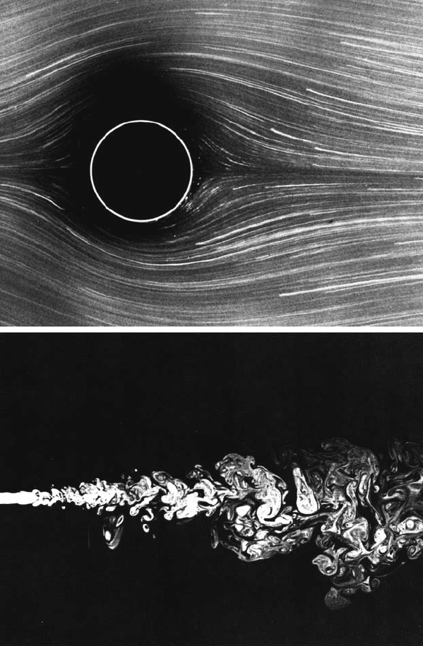
A pictures of the resulting ﬂow at small Reynolds number is shown in the

upper panel of Fig. 6.1. R =1.54 is typical for the laminar ﬂow in the small-

R limit. The ﬂuid ﬂows along the cylinder surface on both sides and closes

behind the cylinder. As the Reynolds number is increased, say in the range

R ∼ 10,...,20, the ﬂow detaches from the cylinder walls at the rear, and

forms two countercirculating eddies. The bottom panel of Fig. 6.1 shows a

rather extreme case (R = 2300) of the opposite limit. At very large Reynolds

numbers, eddies of all sizes form in irregular structures behind the cylinder.

The situation is rather similar to the bottom panel of Figs. 6.1. This picture

shows a turbulent water jet emerging from a nozzle at R ≈ 2300, and has

been preferred for its photographic quality.

The basic equation for ﬂuid ﬂow is the Navier–Stokes equation

∂

v + v · ∇v = −∇P + ν∇

v . (6.2)

The various terms have an immediate interpretation. The left-hand side is

the total derivative dv/dt including two contributions: the explicit acceler-

ation of ﬂuid molecules within a small volume, and the change in velocity

due to the ﬂow, i.e., molecules entering and leaving the small reference vol-

ume with diﬀerent velocities. The ﬁrst term on the right-hand side is the

external force (pressure gradient), and the second term represents friction.

An incompressible ﬂuid, in addition, has

∇ · v =0. (6.3)

It is believed that these two equations are suﬃcient to describe turbulence.

The problem is that there are no explicit solutions, and almost no exact

information on their properties. Much of our information therefore comes

from computer simulations.

6.2 Turbulent Flows 175

Fig. 6.1. Flow past a circular cylinder at R =1.54 (top panel, photograph by S.

Taneda). Turbulent water jet at R ≈ 2300 (bottom panel, photograph by Dimotakis,

Lye, and Papatoniou). Reprinted from M. Van Dyke (ed.): An Album of Fluid

Motion,

1982 Parabolic Press, Stanford

176 6. Turbulence and Foreign Exchange Markets

Here are a few important facts:

• Scaling: With

δv



()=[v(r + ) − v(r)] ·

 (6.4)

being the diﬀerence of the component of the velocity parallel to the ﬂow,

between two points along the ﬂow direction, the structure function

()=δv



()∼

2/3

(6.5)

has power-law scaling with the distance of the points. At the same time,

the same function involving the velocity components perpendicular to the

ﬂow direction scales with the same exponent

δv

⊥

()∼

2/3

. (6.6)

The energy spectrum then scales as

E(k) ∼ k

−5/3

, (6.7)

where k ∼ 

−1

∼ ω is the wavenumber.

• The rate of energy dissipation per unit mass remains ﬁnite even in the limit

of vanishing viscosity:

dε

> 0evenforν → 0 . (6.8)

• Kolmogorov theoretically derived

δv



() = −

ε for R →∞, (6.9)

which represents one of the few exact results on turbulence. It is derived

from the Navier–Stokes equation, assuming in addition homogeneity and

isotropy.

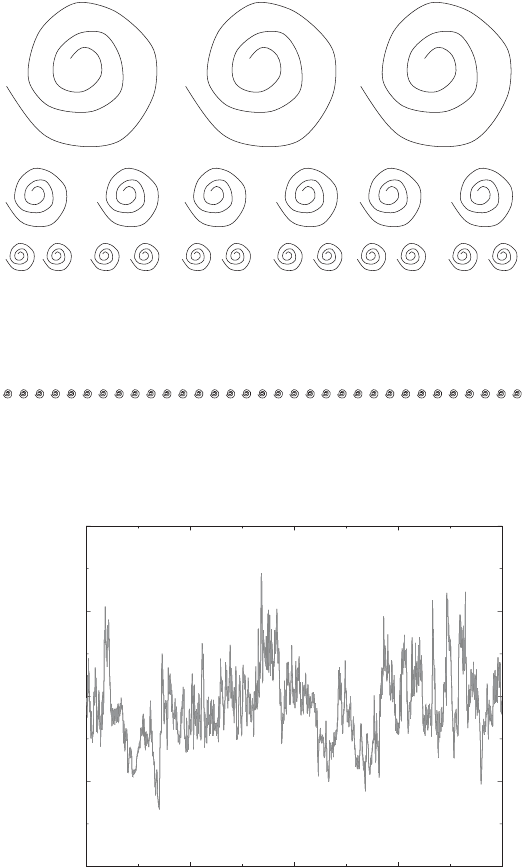
• The cascade idea is illustrated in Fig. 6.2. Here, one starts from the ob-

servation that turbulence generates eddies at many diﬀerent length scales.

One now assumes that external energy is injected into the eddies at the

largest scale of the problem (injection scale). Eddies break up into smaller

eddies which themselves break up into smaller eddies, etc., and energy

is transferred from the big eddies into the small eddies, until one arrives

at the smallest scale where the energy is ﬁnally dissipated. Kolmogorov

and Obhukov have turned this idea into a quantitative model [134] from

which, e.g., the scaling exponents of the various moments of the velocity

diﬀerences, (6.5), (6.6), or (6.9), can be derived.

6.2 Turbulent Flows 177

Fig. 6.2. The cascade idea. Energy is injected at the biggest length scale. Eddies at

that scale break up into smaller eddies, transferring energy to smaller and smaller

scale, until it is dissipated at the smallest scale, the dissipation scale

0.0 5000.0 10000.0 15000.0 20000.0

sampling time (arbitrary units)

velocity (arbitrary units)

0.0

5000.0

10000.0

15000.0

20000.0

Fig. 6.3. Time series of a turbulent ﬂow. The local velocity of a helium jet at low

temperature has been recorded with a hot-wire anemometer. Data provided by J.

Peinke, Universit¨at Oldenburg

178 6. Turbulence and Foreign Exchange Markets

6.2.2 Statistical Description of Turbulence

Some progress can be made by attempting a statistical description of turbu-

lence [135, 136]. Figure 6.3 suggests a close analogy to problems of ﬁnance: it

represents the signal (velocity of the ﬂow) recorded as a function of time, by

a hot-wire anemometer, a local probe in a low-temperature helium jet. These

data are part of the time series used in the statistical analysis of Chabaud et

al., to be discussed below [135]. In the absence of information, it would be

diﬃcult to decide if this is a ﬁnancial time series or not!

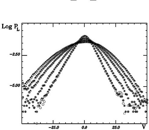
From these time series, one can deduce probability density functions for

the changes of the longitudinal velocity component (6.4) measured on diﬀer-

ent length scales 

[135, 136]. In much the same way, we discussed proba-

bility density functions of the price changes of ﬁnancial assets, measured on

diﬀerent time scales, e.g., Fig. 5.10. Figure 6.4 displays such a set of distrib-

ution functions. For large scales, the probability densities are approximately

Gaussian, while they approach a more exponential distribution as the length

scales are reduced.

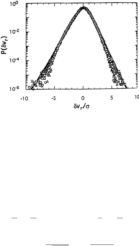
Do these probability densities show scaling? We may rescale the distrib-

utions empirically as (the index  on δv will be dropped from now on)



(δv) →





δv





, (6.10)

Fig. 6.4. Probability density functions of the longitudinal velocity in turbulent

ﬂows at diﬀerent length scales, decreasing from top to bottom in the wings. 

424, 224, 124, 52, 24 from top to bottom with 

= 1024. Circles are data points,

and crosses have been obtained by iteration with the experimentally determined

conditional probability density functions, starting at 

. By courtesy of J. Peinke.

Reprinted from R. Friedrich and J. Peinke: Phys. Rev. Lett. 78, 863 (1997),

1997

by the American Physical Society

6.2 Turbulent Flows 179

Fig. 6.5. Rescaled probability density function for the longitudinal velocity changes

of turbulent ﬂows. The solid line is a ﬁt explained in the text. By courtesy of J.

Peinke. Reprinted from B. Chabaud, et al.: Phys. Rev. Lett. 73, 3227 (1994),

1994

by the American Physical Society

where σ



is the empirical standard deviation at length scale .Asshown

in Fig. 6.5, all data now more or less collapse onto a single master curve,

demonstrating that they obey the same basic laws, and are only distinguished

by the diﬀerent length scales of the measurement. The master curve has

some similarity to a Gaussian in its center and is more like an exponential

distribution in the wings. While there is no simple expression, it can be

described as an integral over a continuous family of Gaussians [135]





δv







∞

−∞

d ln σG



(ln σ)





δv



(6.11)

with



(ln σ)=



2πλ()

exp



−

σ/σ



2λ()



. (6.12)

Notice that the empirical distribution function at the largest length scale,



, is nearly Gaussian. The probability distribution at a smaller length scale

<

is therefore represented by a weighted integral over Gaussians whose

standard deviations are log-normally distributed. This integral over Gaus-

sians describes the curves extremely well. The standard deviations σ



are

scale dependent through the width λ() of their distribution, and generate

themselves from those on bigger length scales. This directly implements the

cascade idea. However, Kolmogorov’s theory predicts that λ ∝−ln(/

)

which is not observed in the experiment.