Tsoulfanidis N. Measurement and detection of radiation
Подождите немного. Документ загружается.

348
MEASUREMENT
AND
DETECTION
OF
RADIATION
the study of events in terms of more than one parameter. Such requirements
occur in
1.
Coincidence measurements where the energy spectrum from both detectors
need be analyzed
2. Simultaneous measurement of energy and mass distribution of fission frag-
ments
3. Study of energy and angular dependence of nuclear reactions involving many
particles, etc.
The "direct7' method of multiparameter analysis would be to use an ar-
rangement such that all parameters but one are limited to a narrow range (by
using a single-channel analyzer) and the remaining parameter is recorded by an
MCA.
After an adequate number of events have been recorded, the value of
one of the fixed parameters is changed, and the measurement is repeated. This
process continues until all values of all parameters are covered. Obviously, such
an approach is cumbersome and time consuming.
A
more efficient way of performing the measurement is by storing the
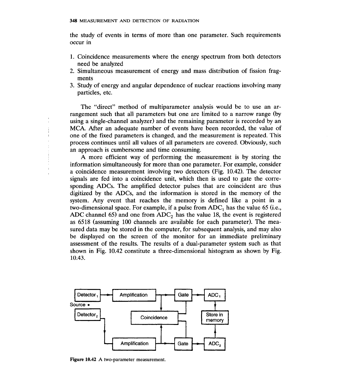
information simultaneously for more than one parameter. For example, consider
a coincidence measurement involving two detectors (Fig. 10.42). The detector
signals are fed into a coincidence unit, which then is used to gate the corre-
sponding ADCs. The amplified detector pulses that are coincident are thus
digitized by the
ADCs, and the information is stored in the memory of the
system. Any event that reaches the memory is defined like a point in a
two-dimensional space. For example, if a pulse from ADC, has the value 65
(i.e.,
ADC channel 65) and one from ADC, has the value 18, the event is registered
as 6518 (assuming 100 channels are available for each parameter). The mea-
sured data may be stored in the computer, for subsequent analysis, and may also
be displayed on the screen of the monitor for an immediate preliminary
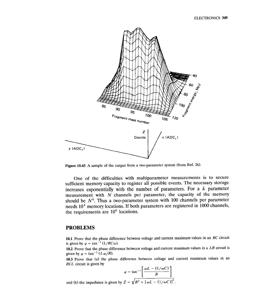
assessment of the results. The results of a dual-parameter system such as that
shown in Fig. 10.42 constitute a three-dimensional histogram as shown by Fig.
10.43.
Amplification Gate
Source
I
F$
Coincidence
1-1
Amplification Gate ADC,
Figure
10.42
A
two-parameter measurement.
ELECTRONICS
349
Counts
x
(ADC,)
y
(ADC,)
Figure
10.43
A
sample of the output from a two-parameter system (from Ref.
26).
One of the difficulties with multiparameter measurements is to secure
sufficient memory capacity to register all possible events. The necessary storage
increases exponentially with the number of parameters. For a
k
parameter
measurement with
N
channels per parameter, the capacity of the memory
should be
N~.
Thus a two-parameter system with
100
channels per parameter
needs
lo4
memory locations.
If
both parameters are registered in
1000
channels,
the requirements are
lo6
locations.
PROBLEMS
10.1 Prove that the phase difference between voltage and current maximum values in an RC circuit
is given by
q
=
tan-' (l/RCw).
10.2 Prove that the phase difference between voltage and current maximum values in a LR circuit is
given by
cp
=
tan-' (Lo/R).
10.3 Prove that (a) the phase difference between voltage and current maximum values in an
RCL circuit is given by
cp
=
tan-'
[
wL
-
YC)
I
and (b) the impedance is given by Z
=
JR'
+
[
wL
-
(l/d)12 .
350
MEASUREMENT AND DETECTION
OF
RADIATION
10.4
Prove that the output signal of a differentiating circuit is, for a step input, equal to
V,(t)
=
Ke-'IRC
10.5
Show that the output signal of a differentiating circuit is given by
when the input signal is given by
&(t)
=
K~/T.
10.6
Show that the output signal of an integrating circuit is, for a step input, equal to
10.7
Show that the output signal of
a
differentiating circuit is given by
when the input signal is
&(1
-
e-'/').
10.8
A
coincidence measurement has to be performed within a time
T.
Show that the standard
deviation of the true coincidence rate is given by
where
r,
=
accidental coincidence rate
r,
=
true coincidence rate
BIBLIOGRAPHY
Kowalski, E.,
Nuclear Electronics,
Springer-Verlag, New York,
1970.
Malmstadt, H.
V.,
Enke,
C.
G., and Toren, E.
C.,
Electronics for Scientists,
W.
A.
Benjamin, New
York,
1963.
Nicholson,
P.
W.,
Nuclear Electronics,
Wiley, London,
1974.
REFERENCES
1.
Chase, R. L.,
Rev. Sci. Instrum.
391318 (1968).
2.
Gedcke, D.
A.,
and McDonald, W.
J.,
Nucl. Znstrum. Meth.
55:377 (1967).
3.
Maier, M.
R.,
and Sperr,
P.,
Nucl. Instrum. Meth.
87:13 (1970).
4.
Strauss, M. G., Larsen,
R.
N., and Sifter, L. L.,
Nucl. Instrum. Meth.
46:45 (1967).
5.
Graham, R.
L.,
Mackenzie,
I.
K., and Ewan, G.
T.,
ZEEE Trans. NS 13
1:72 (1966).
6.
Viencent,
C.
H.,
Nucl. Instrum. Meth.
127:421 (1975).
7.
Smith, D.,
Nucl. Znstrum. Meth.
152:505 (1978).
8.
Kuchnir,
F.
T.,
and Lynch,
F.
J.,
IEEE Trans. NS
15
3:107 (1968).
9.
Alexander,
T.
K., and Goulding,
F.
S.,
Nucl. Znstrum. Meth.
13:244 (1961).
10.
Heistek,
L.
J.,
and Van der Zwan,
L.,
Nucl. Instrum. Meth.
80:213 (1970).
11.
McBeth, G. W., Lutkin,
J.
E., and Winyard,
R.
A,,
Nucl. Instrum. Meth.
93:99 (1971).
12.
Brooks,
F.
D.,
Nucl. Znstrum. Meth.
4151 (1959).
13.
Kinbara, S., and Kumahara,
T.,
Nucl. Instrum. Meth.
70:173 (1969).
14.
Burrus,
W.
R.,
and Verbinski, V.
V.,
Nucl. Instrum. Meth.
67:181 (1969).
ELECTRONICS 351
15.
Verbinski, V. V., Burrus,
W.
R.,
Love,
T.
A,,
Zobel, W., and Hill,
N.
W.,
Nucl. Instrum. Meth.
653 (1968).
16.
Fortt, M., Konsta,
A,,
and Moranzana,
C.,
Electronic Methods for Discrimination of Scintillation
Shapes
(IAEA
Conf. Nucl. Electr. Belgrade,
1961) NE-59.
17.
Brenner,
R.,
Rev. Sci. Instrum.
40:1011 (1969).
18.
Nowlin, C.
H.,
and Blankenship,
J.
L.,
Rev. Sci. Instrum.
36:1830 (1965).
19.
Fairstein,
E.,
and Hahn,
J.,
Nucleonics
23,
no.
7:56 (1965).
20.
Fairstein,
E.,
and Hahn, J.,
Nucleonics
23,
9:81 (1965).
21.
Fairstein, E., and Hahn,
J.,
Nucleonics
23,
no.
11:50 (1965).
22.
Fairstein, E., and Hahn,
J.,
Nucleonics
24,
no.
1:54 (1966).
23.
Fairstein, E., and Hahn,
J.,
Nucleonics
24,
no.
3:68 (1966).
24.
Wilkinson,
D.
H.,
Philos. Soc.
46508 (1950).
25.
Canberra Industries, Inc.,
Edition Nine, Instruments Catalog,
Meriden, CT,
1993.
26.
Diorio,
G.,
and Wehring,
B.
W.,
Nucl. Instrum. Meth.
147:487 (1977).


CHAPTER
ELEVEN
DATA
ANALYSIS
METHODS
11.1
INTRODUCTION
Rawt experimental data seldom give the answer to the problem that is the
objective of the measurement. In most cases, additional calculations or analysis
of the raw data is necessary. The analysis of the raw data may consist of a simple
division of the counts recorded in a scaler by the counting time to obtain
counting rates, may require fitting an analytical function to the data, or may
necessitate unfolding of a measured spectrum.
Whatever the analysis of the data may entail, there are some general
methods helpful to the analyst. The objective of this chapter is to present a brief
introduction to these general methods and principles of data analysis.
11.2
CURVE FITTING
The results of most experiments consist of a finite number of values (and their
errors) of a dependent variable
y
measured as a function of the independent
variable
x
(Fig.
11.1).
The objective of the measurement of
y
=
y(x)
may be one
'~aw data consist of the numbers obtained by the measuring device, e.g., a scaler, a clock,
or
a
voltmeter.
354
MEASUREMENT
AND
DETECTION OF RADIATION
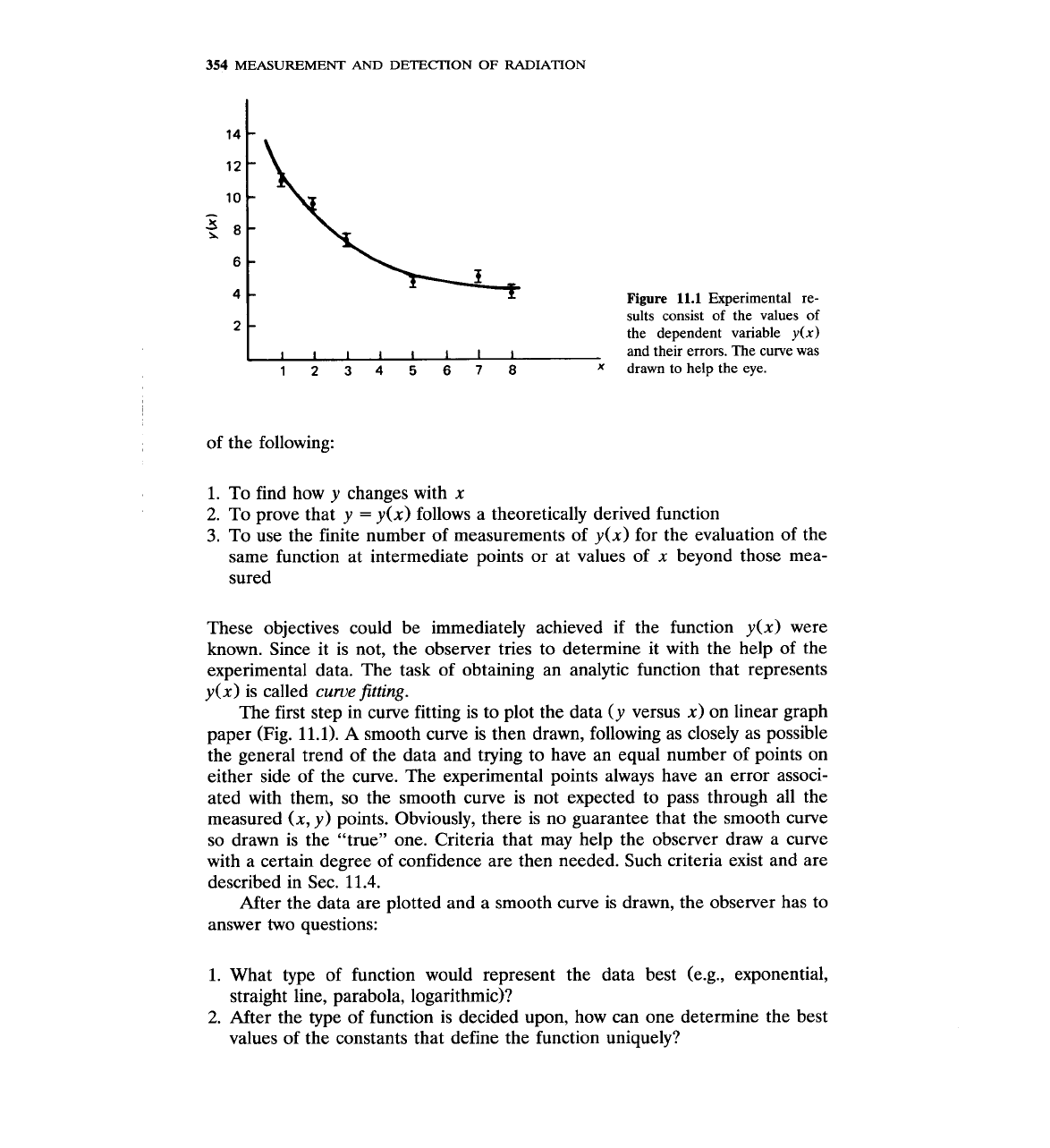
Figure
11.1
Experimental re-
sults consist of the values of
the dependent variable
y(x)
and their errors. The curve was
12345678
x
drawn to help the eye.
of the following:
1.
To find how y changes with x
2.
To prove that y
=
y(x) follows a theoretically derived function
3.
To use the finite number of measurements of y(x) for the evaluation of the
same function at intermediate points or at values of x beyond those mea-
sured
These objectives could be immediately achieved if the function y(x) were
known. Since it is not, the observer tries to determine it with the help of the
experimental data. The task of obtaining an analytic function that represents
y(x) is called
cume
fitting.
The first step in curve fitting is to plot the data (y versus x) on linear graph
paper (Fig. 11.1).
A
smooth curve is then drawn, following as closely as possible
the general trend of the data and trying to have an equal number of points on
either side of the curve. The experimental points always have an error associ-
ated with them, so the smooth curve is not expected to pass through all the
measured
(x, y) points. Obviously, there is no guarantee that the smooth curve
so drawn is the "true7' one. Criteria that may help the observer draw a curve
with a certain degree of confidence are then needed. Such criteria exist and are
described in Sec.
11.4.
After the data are plotted and a smooth curve is drawn, the observer has to
answer two questions:
1. What type of function would represent the data best (e.g., exponential,
straight line, parabola, logarithmic)?
2.
After the type of function is decided upon, how can one determine the best
values of the constants that define the function uniquely?
DATA
ANALYSIS
METHODS
355
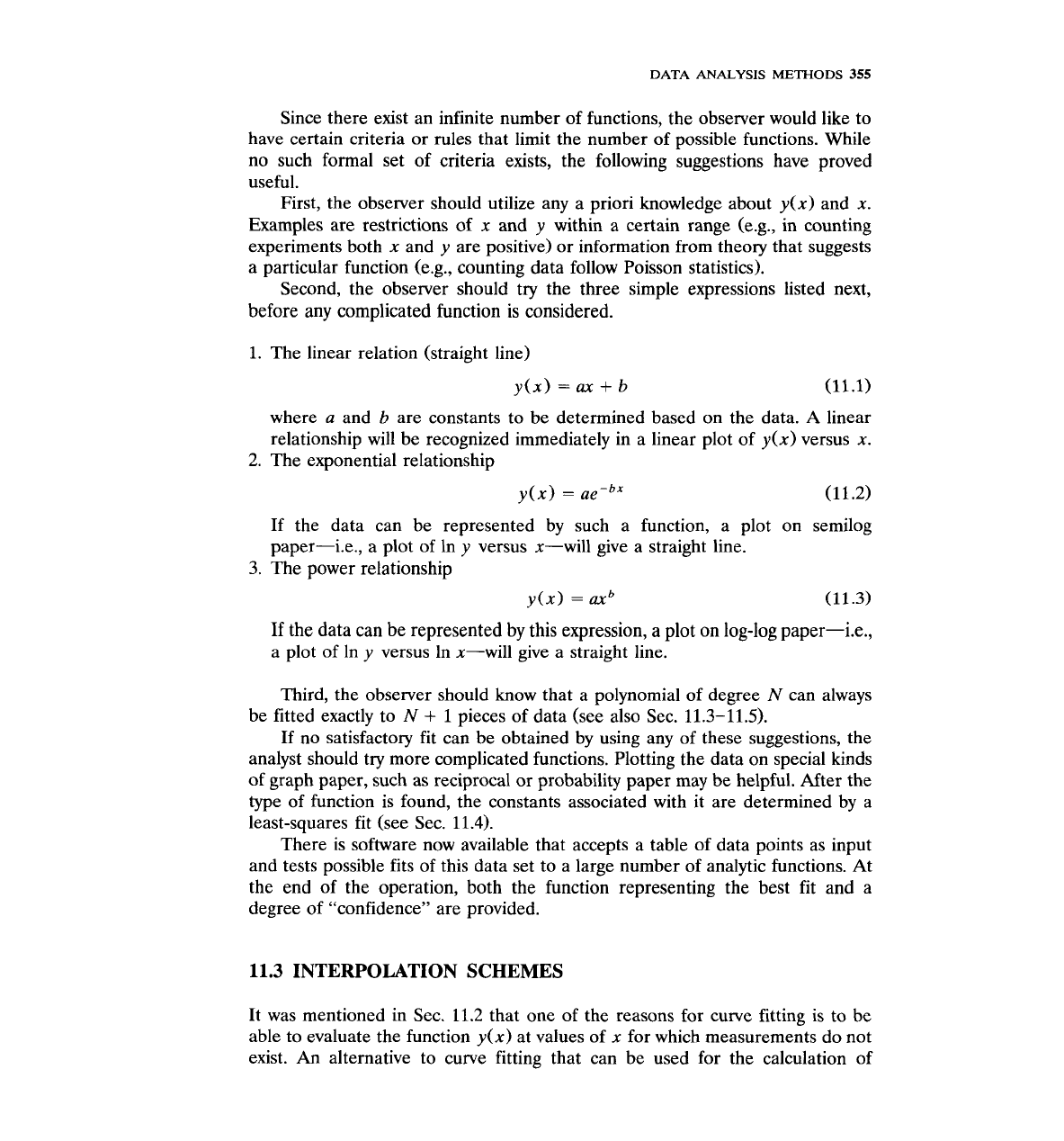
Since there exist an infinite number of functions, the observer would like to
have certain criteria or rules that limit the number of possible functions. While
no such formal set of criteria exists, the following suggestions have proved
useful.
First, the observer should utilize any a priori knowledge about
y(x) and x.
Examples are restrictions of
x
and
y
within a certain range (e.g., in counting
experiments both x and y are positive) or information from theory that suggests
a particular function (e.g., counting data follow Poisson statistics).
Second, the observer should try the three simple expressions listed next,
before any complicated function is considered.
1.
The linear relation (straight line)
where
a
and
b
are constants to be determined based on the data.
A
linear
relationship will be recognized immediately in a linear plot of y(x) versus
x.
2.
The exponential relationship
If the data can be represented by such a function, a plot on semilog
paper-i.e., a plot of In
y
versus x-will give a straight line.
3. The power relationship
If
the data can be represented by this expression, a plot on log-log paper-i.e.,
a plot of In y versus In x-will give a straight line.
Third, the observer should know that a polynomial of degree
N
can always
be fitted exactly to
N
+
1
pieces of data (see also Sec. 11.3-11.5).
If no satisfactory fit can be obtained by using any of these suggestions, the
analyst should try more complicated functions. Plotting the data on special kinds
of graph paper, such as reciprocal or probability paper may be helpful. After the
type of function is found, the constants associated with it are determined by a
least-squares fit (see
Sec. 11.4).
There is software now available that accepts a table of data points as input
and tests possible fits of this data set to a large number of analytic functions. At
the end of the operation, both the function representing the best fit and a
degree of "confidence" are provided.
11.3
INTERPOLATION SCHEMES
It was mentioned in Sec. 11.2 that one of the reasons for curve fitting is to be
able to evaluate the function y(x) at values of x for which measurements do not
exist.
An
alternative to curve fitting that can be used for the calculation of

356
MEASUREMENT
AND
DETECTION
OF
RADIATION
intermediate y(x) values is the method of interpolation. This section presents
one of the basic interpolation techniques-the Lagrange formula. Many other
formulas exist that the reader can find in the bibliography of this chapter (e.g.,
see Hildebrand, and Abramowitz and Stegan's Handbook
or
Mathematical Func-
tions).
Assume that N values of the dependent variable y(x) are known at the N
points
xi, x,
I
xi
I
x, for
i
=
1,.
. .
,
N.
The pairs of data (yi, xi) for i
=
1,.
. .
,
N, where y(xi)
=
yi, may be the results of an experiment or tabulated
values. Interpolation means to obtain a value y(x) for x,
<
x
<
x, based on the
data (y,, xi), when the point x is not one of the
N
values for which y(x) is
known.
The
Lagrange interpolation formula expresses the value y(x) in terms of
polynomials (up to degree N
-
1
for N pairs of data). The general equation is
where
The error associated with
Eq.
11.4 is given by
where yM+'(() is the (M
+
1) derivative of y(x) evaluated at the point
5,
x,
<
6
<
x,. Since y(x) is not known analytically, the derivative in Eq.
11.6
has to be calculated numerically.
Equation 11.4 is the most general. It uses all the available points to
calculate any new value of y(x) for x,
<
x
<
x,. In practice, people use only a
few points at a time, as the following two examples show.
Example
11.1
Derive the Lagrange formula for
M
=
1.
Answer
If M
=
1,
Eq.
11.4 takes the form (also using Eq. 11.5)
where yi
=
y(xi). The points x, and x, could be anywhere between x, and x,,
but the point
x
should be xo
I
x
I
x,.
DATA ANALYSIS
METHODS
357
To calculate
y(x)
at any
x,
Eq.
11.7
uses two points, one on either side of
x,
and for this reason it is called the
Lagrange two-point interpolation formula.
Equation
11.7
may be written in the form
which shows that the two-point formula amounts to a linear interpolation.
The error associated with the two-point formula is obtained from Eq.
11.6:
where
5
)
is the second derivation evaluated at
5,
x,
5
5
<
x,.
Example
11.2
Derive the Lagrange formula for
M
=
2.
Answer
If
M
=
2,
Eq.
11.4
takes the form
To calculate
y(x)
at any point
x,
Eq.
11.9
uses three points
xo, x,, x2
with
x,
I
x
I
x,,
and is called the
Lagrange three-point interpolation formula.
The
three-point formula amounts to a parabolic representation of the function
y(x)
between any three points.
The error associated with the three-point formula is (applying again
Eq.
11.6):
where
yC3)(5)
is the third derivative evaluated at
5,
x,
5
5
<
x,.
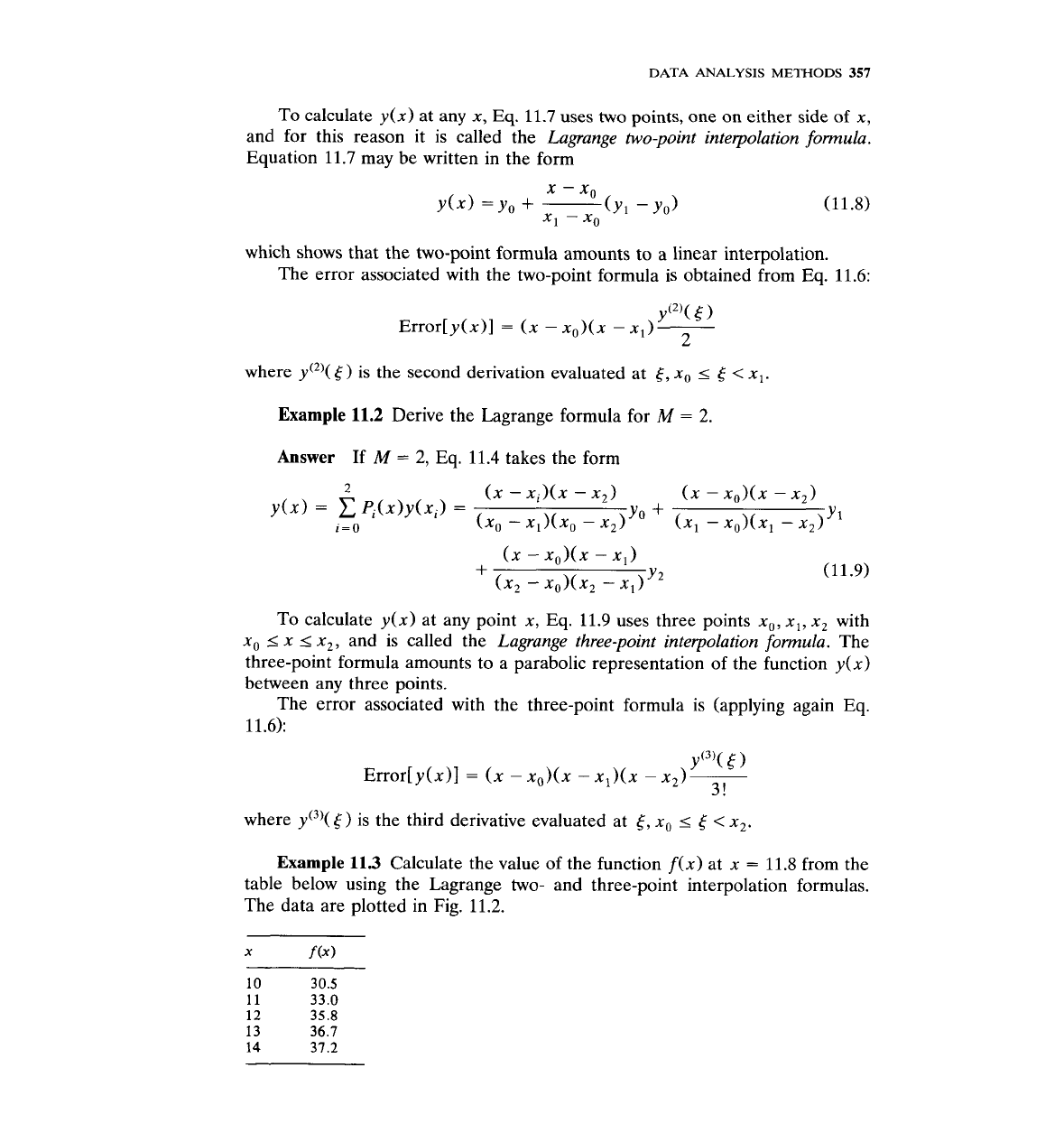
Example
11.3
Calculate the value of the function
f(x)
at
x
=
11.8 from the
table below using the Lagrange two- and three-point interpolation formulas.
The
data are plotted in Fig.
11.2.