Tsoulfanidis N. Measurement and detection of radiation

Подождите немного. Документ загружается.

328

MEASUREMENT

AND

DETECTION OF RADIATION

circuits

Figure

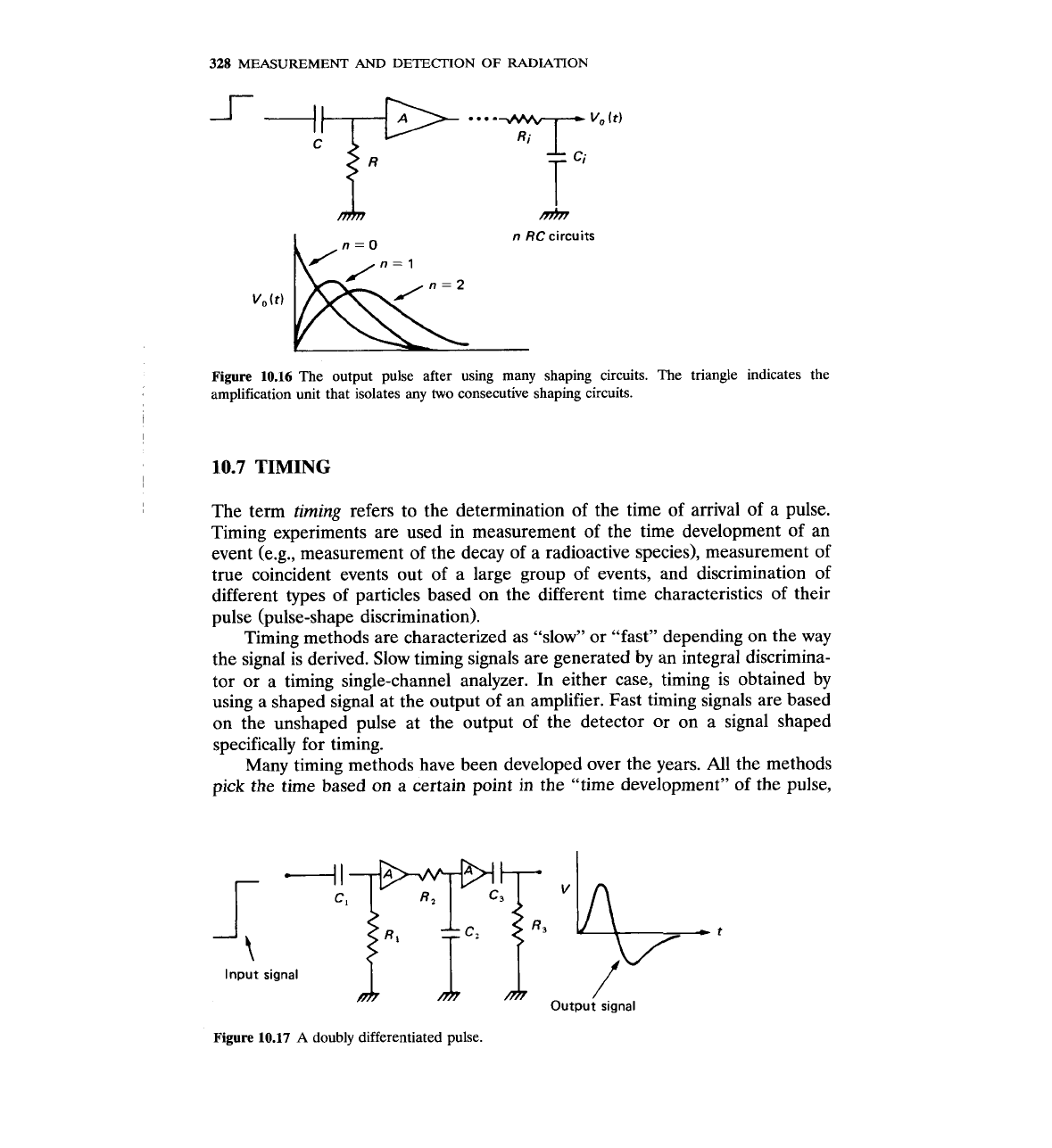
10.16 The output pulse after using many shaping circuits. The triangle indicates the

amplification unit that isolates any two consecutive shaping circuits.

10.7

TIMING

The term

timing

refers to the determination of the time of arrival of a pulse.

Timing experiments are used in measurement of the time development of an

event (e.g., measurement of the decay of a radioactive species), measurement of

true coincident events out of a large group of events, and discrimination of

different types of particles based on the different time characteristics of their

pulse (pulse-shape discrimination).

Timing methods are characterized as "slow" or "fast" depending on the way

the signal is derived. Slow timing signals are generated by an integral discrimina-

tor or a timing single-channel analyzer. In either case, timing is obtained by

using a shaped signal at the output of an amplifier. Fast timing signals are based

on the unshaped pulse at the output of the detector or on a signal shaped

specifically for timing.

Many timing methods have been developed over the years. All the methods

pick

the time based on a certain point in the "time development" of the pulse,

Figure

10.17

doubly differentiated pulse.

ELECTRONICS

329

polar

pulse

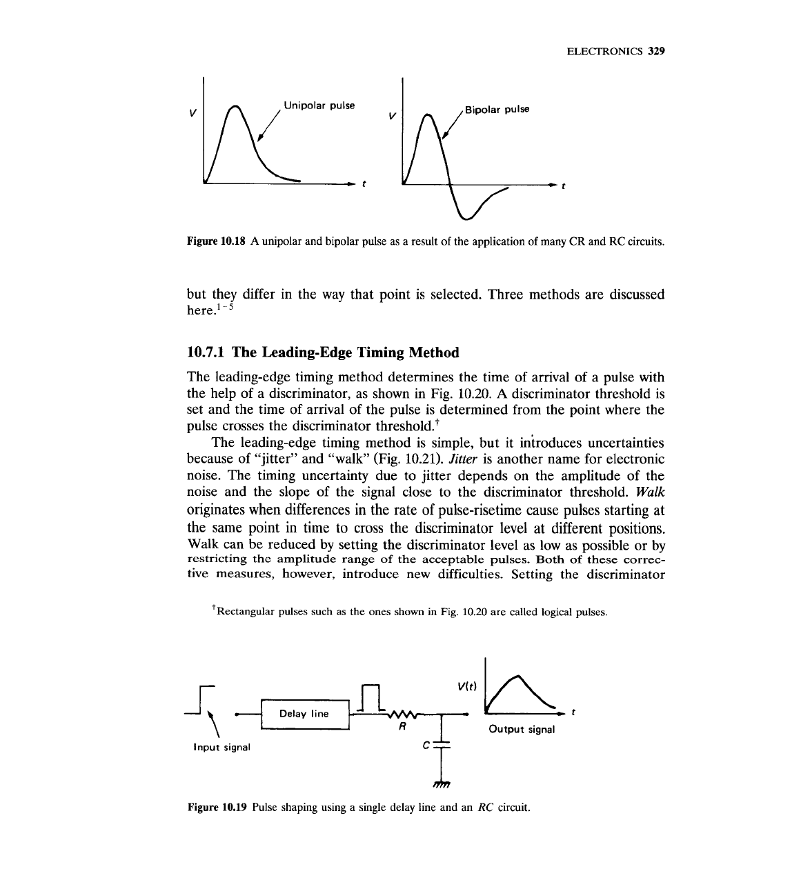
Figure 10.18

unipolar and bipolar pulse as a result of the application of many CR and RC circuits.

but they differ in the way that point is selected. Three methods are discussed

here.'

10.7.1

The Leading-Edge Timing Method

The leading-edge timing method determines the time of arrival of a pulse with

the help of a discriminator, as shown in Fig. 10.20.

discriminator threshold is

set and the time of arrival of the pulse is determined from the point where the

pulse crosses the discriminator threshold.+

The leading-edge timing method is simple, but it introduces uncertainties

because of "jitter" and "walk (Fig. 10.21).

Jitter

is another name for electronic

noise. The timing uncertainty due to jitter depends on the amplitude of the

noise and the slope of the signal close to the discriminator threshold.

Walk

originates when differences in the rate of pulse-risetime cause pulses starting at

the same point in time to cross the discriminator level at different positions.

Walk can be reduced by setting the discriminator level as low as possible or by

restricting the amplitude range of

the

acceptable pulses.

Both

of these correc-

tive measures, however, introduce new difficulties. Setting the discriminator

t~ectangular pulses such as the ones shown

Fig.

10.20

are called logical pulses.

Delay line

Output

signal

Input signal

Figure 10.19

Pulse shaping using a single delay line and an

circuit.

330

MEASUREMENT

AND

DETECTION

RADIATION

Discriminator output

Time

arrival

pulse

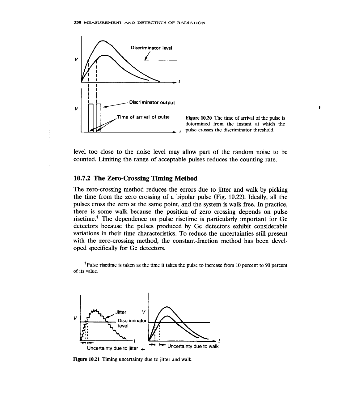
Figure

10.20

The time of arrival of the pulse is

determined from the instant at which the

pulse crosses the discriminator threshold.

level too close to the noise level may allow part of the random noise to be

counted. Limiting the range of acceptable pulses reduces the counting rate.

10.7.2

The Zero-Crossing Timing Method

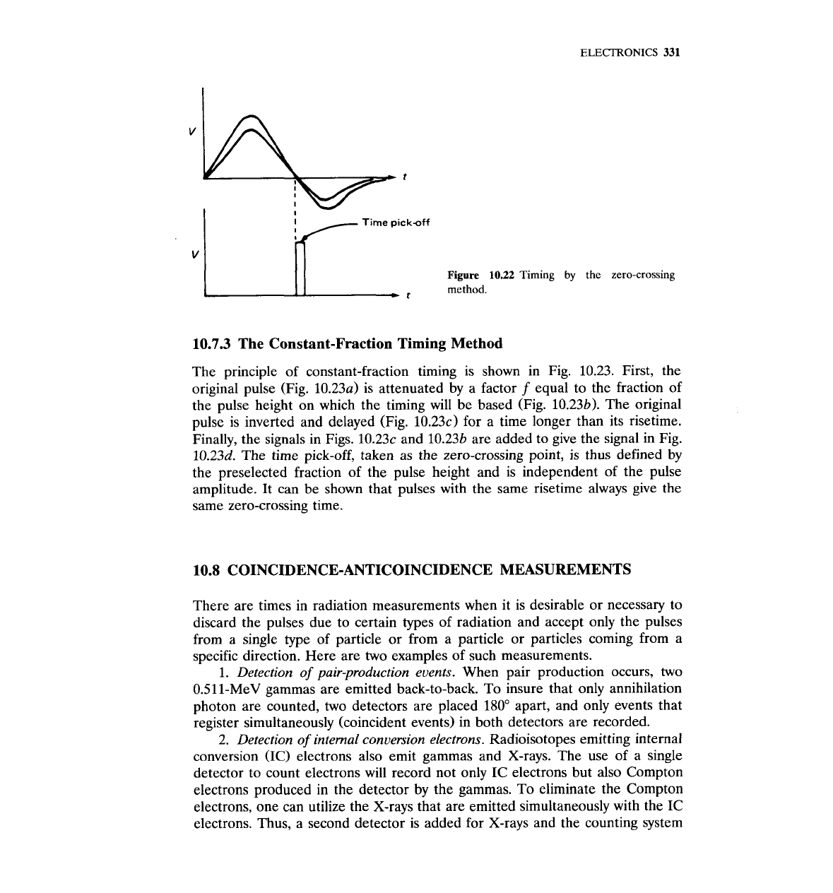
The zero-crossing method reduces the errors due to jitter and walk by picking

the time from the zero crossing of a bipolar pulse (Fig.

10.22).

Ideally, all the

pulses cross the zero at the same point, and the system is walk free.

practice,

there is some walk because the position of zero crossing depends on pulse

risetime.+ The dependence on pulse risetime is particularly important for Ge

detectors because the pulses produced by Ge detectors exhibit considerable

variations in their time characteristics. To reduce the uncertainties still present

with the zero-crossing method, the constant-fraction method has been devel-

oped specifically for Ge detectors.

'Pulse risetime is taken as the time it takes the pulse to increase from

percent to

percent

of its value.

Jitter

Discriminator

level

Uncertainty due

jitter

buncertainty due to walk

Figure

10.21

Timing uncertainty due to jitter and walk.

Time

pickaff

Figure

10.22

Timing

the zero-crossing

method.

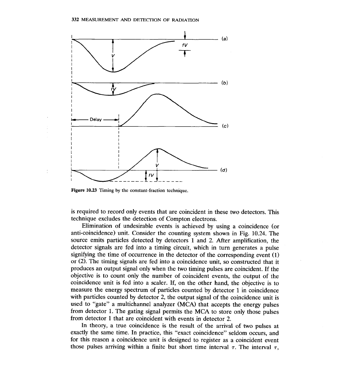
10.7.3 The Constant-Fraction Timing Method

The principle of constant-fraction timing is shown in Fig. 10.23. First, the

original pulse (Fig. 10.23a) is attenuated by a factor

equal to the fraction of

the pulse height on which the timing will be based (Fig. 10.23b). The original

pulse is inverted and delayed (Fig. 10.23~) for a time longer than its risetime.

Finally, the signals in Figs. 10.23~ and 10.23b are added to give the signal in Fig.

10.23d. The time pick-off, taken as the zero-crossing point, is thus defined by

the preselected fraction of the pulse height and is independent of the pulse

amplitude. It can be shown that pulses with the same risetime always give the

same zero-crossing time.

10.8 COINCIDENCE-ANTICOINCIDENCE MEASUREMENTS

There are times in radiation measurements when it is desirable or necessary to

discard the pulses due to certain types of radiation and accept only the pulses

from a single type of particle or from a particle or particles coming from a

specific direction. Here are two examples of such measurements.

1. Detection of pair-production events. When pair production occurs, two

0.511-MeV gammas are emitted back-to-back. To insure that only annihilation

photon are counted, two detectors are placed

180"

apart, and only events that

2. Detection of internal conversion electrons. Radioisotopes emitting internal

conversion

(IC)

electrons also emit gammas and X-rays. The use of a single

detector to count electrons will record not only IC electrons but also Compton

electrons produced in the detector by the gammas. To eliminate the Compton

electrons, one can utilize the X-rays that are emitted simultaneously with the IC

electrons. Thus, a second detector is added for X-rays and the counting system

332

MEASUREMENT

AND

DETECTION OF RADIATION

Figure

10.23

Timing

the constant-fraction technique.

is required to record only events that are coincident in these two detectors. This

technique excludes the detection of Compton electrons.

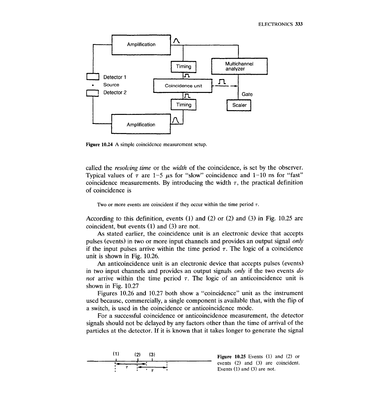
Elimination of undesirable events is achieved by using a coincidence (or

anti-coincidence) unit. Consider the counting system shown in Fig. 10.24. The

source emits particles detected by detectors

and 2. After amplification, the

detector signals are fed into a timing circuit, which in turn generates a pulse

signifying the time of occurrence in the detector of the corresponding event (1)

(2).

The timing signals are fed into a coincidence unit, so constructed that it

produces an output signal only when the two timing pulses are coincident. If the

objective is to count only the number of coincident events, the output of the

coincidence unit is fed into a scaler. If, on the other hand, the objective is to

measure the energy spectrum of particles counted by detector

in coincidence

with particles counted by detector 2, the output signal of the coincidence unit is

used to "gate" a multichannel analyzer (MCA) that accepts the energy pulses

from detector

The gating signal permits the MCA to store only those pulses

from detector

that are coincident with events in detector

In theory, a true coincidence

the result of the arrival of two pulses at

exactly the same time. In practice, this "exact coincidence" seldom occurs, and

for this reason a coincidence unit is designed to register as a coincident event

those pulses arriving within a finite but short time interval

The interval

Amplification

Multichannel

Detector

Source

Coincidence unit

Detector

Figure

10.24

simple coincidence measurement setup.

called the

resolving time

or the

width

of the coincidence, is set by the observer.

Typical values of

are 1-5 ps for "slow" coincidence and 1-10 ns for "fast"

coincidence measurements.

introducing the width

the practical definition

of coincidence is

Two or more events are coincident

they occur within the time period

According to this definition, events

(1)

and

(2)

or (2) and

(3)

in Fig. 10.25 are

coincident, but events (1) and

(3)

are not.

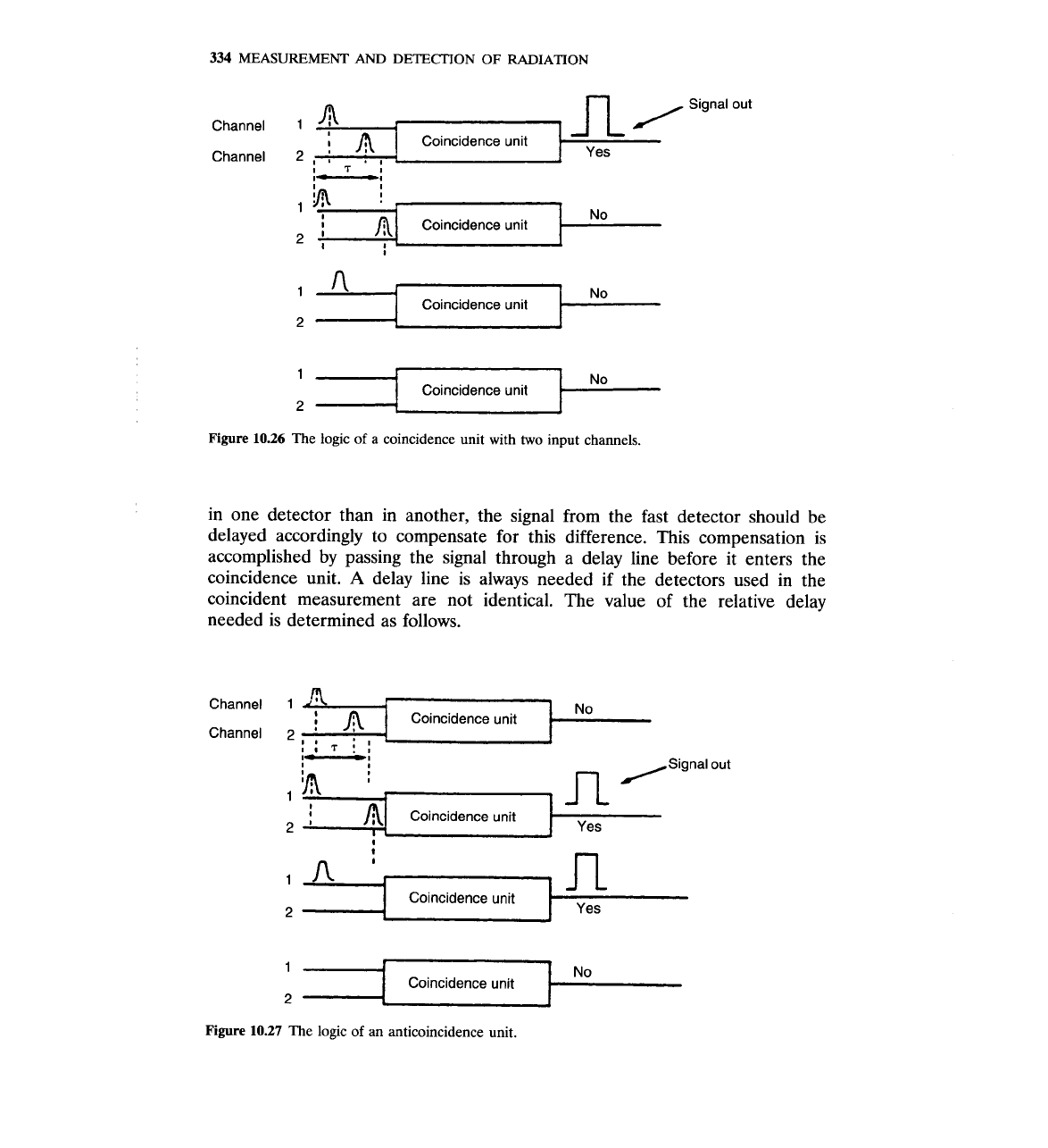
As stated earlier, the coincidence unit is an electronic device that accepts

pulses (events) in two or more input channels and provides an output signal

only

the input pulses arrive within the time period

The logic of a coincidence

unit is shown in Fig. 10.26.

anticoincidence unit is an electronic device that accepts pulses (events)

in two input channels and provides an output signals

only

if the two events

not

arrive within the time period

The logic of an anticoincidence unit is

shown in Fig. 10.27

Figures 10.26 and 10.27 both show a "coincidence" unit as the instrument

used because, commercially, a single component is available that, with the flip of

a switch, is used in the coincidence or anticoincidence mode.

For a successful coincidence or anticoincidence measurement, the detector

signals should not be delayed by any factors other than the time of arrival of the

particles at the detector. If it is known that it takes longer to generate the signal

(1)

(2)

(3)

Figure 10.25

Events

(1)

and (2) or

I-

-a

events (2) and

(3)

are coincident.

Events

(1)

and

(3)

are not.

334

MEASUREMENT

AND DETECTION OF RADIATION

Channel

Signal out

Yes

17,

Coincidence unit

Figure

10.26 The logic of a coincidence unit with two input channels.

in one detector than in another, the signal from the fast detector should be

delayed accordingly to compensate for this difference. This compensation is

accomplished by passing the signal through a delay line before it enters the

coincidence unit.

delay line is always needed if the detectors used in the

coincident measurement are not identical. The value of the relative delay

needed is determined as follows.

Coincidence unit

Yes

Coincidence unit

Figure

10.27 The logic of an anticoincidence unit.

ELECTRONICS

335

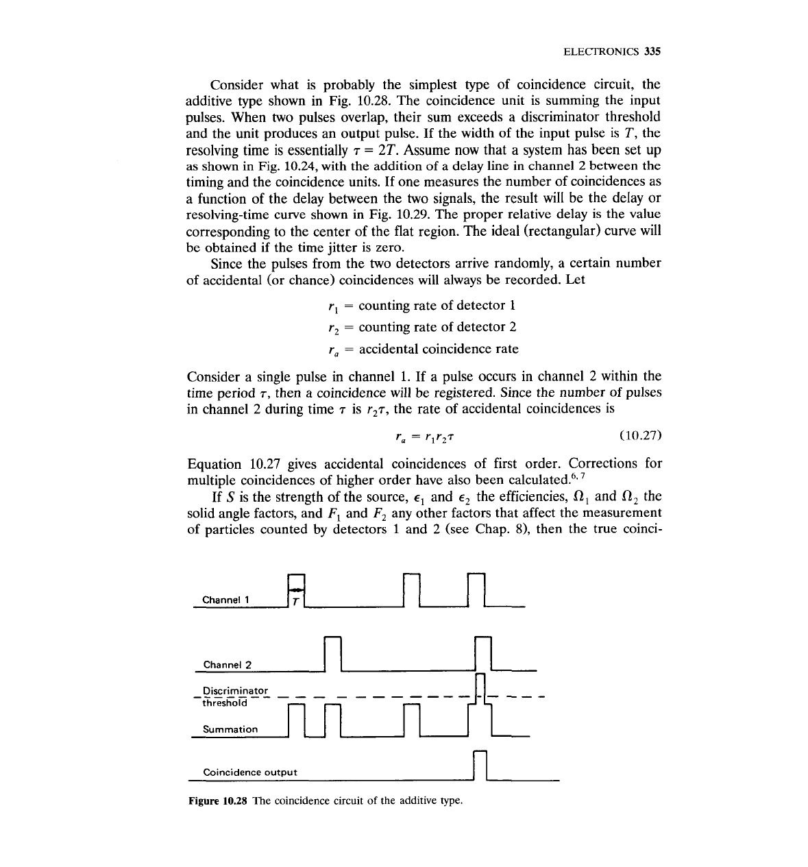
Consider what is probably the simplest type of coincidence circuit, the

additive type shown in Fig. 10.28. The coincidence unit is summing the input

pulses. When two pulses overlap, their sum exceeds a discriminator threshold

and the unit produces an output pulse. If the width of the input pulse is

the

resolving time is essentially

2T.

Assume now that a system has been set

as shown in Fig. 10.24, with the addition

a delay line in channel 2 between the

timing and the coincidence units. If one measures the number of coincidences as

a function of the delay between the two signals, the result will be the delay or

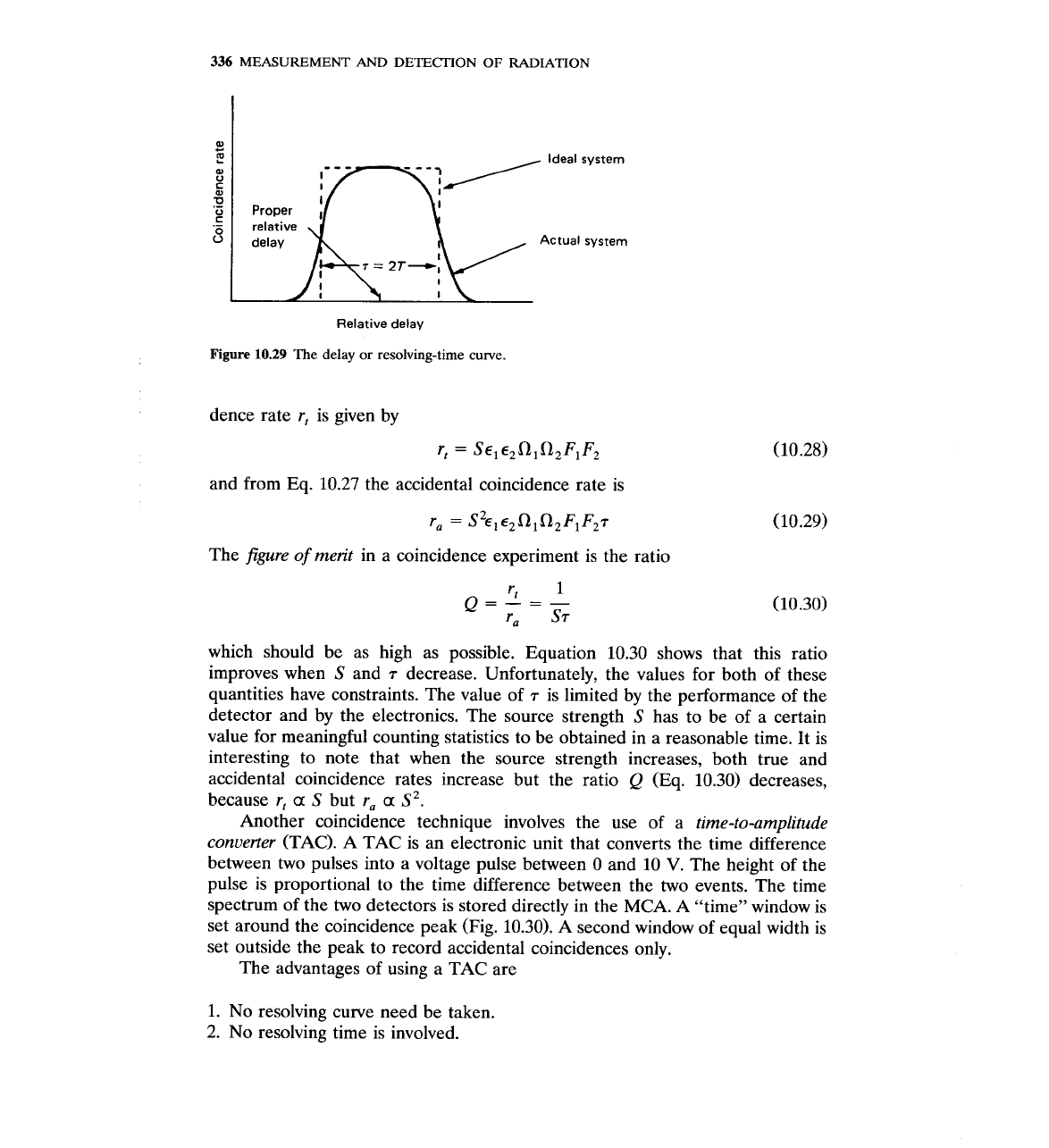
resolving-time curve shown in Fig. 10.29. The proper relative delay is the value

corresponding to the center of the flat region. The ideal (rectangular) curve will

be obtained if the time jitter is zero.

Since the pulses from the two detectors arrive randomly, a certain number

of accidental (or chance) coincidences will always be recorded. Let

counting rate of detector

counting rate of detector 2

accidental coincidence rate

Consider a single pulse in channel 1. If a pulse occurs in channel

within the

time period

then a coincidence will be registered. Since the number of pulses

in channel 2 during time

is r,r, the rate of accidental coincidences is

Equation 10.27 gives accidental coincidences of first order. Corrections for

multiple coincidences of higher order have also been ~alculated.~.

is the strength of the source,

and

the efficiencies,

and R, the

solid angle factors, and

and

any other factors that affect the measurement

of particles counted by detectors

and 2 (see Chap. 8), then the true coinci-

Channel

threshold

Summation

Coincidence output

Figure

10.28

The coincidence circuit

the additive type.

336

MEASUREMENT

AND

DETECTION

RADIATION

Proper

relative

delay

Relative delay

Figure

10.29

The delay or resolving-time

curve.

dence rate

is given by

and from Eq. 10.27 the accidental coincidence rate is

The

Jigure of merit

in a coincidence experiment is the ratio

which should be as high as possible. Equation 10.30 shows that this ratio

improves when

and

decrease. Unfortunately, the values for both of these

quantities have constraints. The value of

is limited by the performance of the

detector and by the electronics. The source strength

has to be of a certain

value for meaningful counting statistics to be obtained in a reasonable time. It is

interesting to note that when the source strength increases, both true and

accidental coincidence rates increase but the ratio

(Eq. 10.30) decreases,

because

but

S2.

Another coincidence technique involves the use of a

time-to-amplitude

converter

(TAC). A TAC is an electronic unit that converts the time difference

between two pulses into

voltage pulse between 0 and 10

The height of the

pulse is proportional to the time difference between the two events. The time

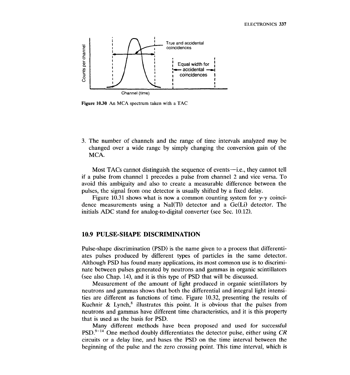
spectrum of the two detectors is stored directly in the MCA. A "time" window is

set around the coincidence peak (Fig. 10.30). A second window of equal width is

set outside the peak to record accidental coincidences only.

The advantages of using a TAC are

No resolving curve need be taken.

2. No resolving time is involved.

ELECTRONICS

337

Equal

width

for

I-

accidental

-1

coincidences

Channel

(time)

Figure

1030

MCA

spectrum taken with a

TAC

The number of channels and the range of time intervals analyzed may be

changed over a wide range by simply changing the conversion gain of the

MCA.

Most TACs cannot distinguish the sequence of events-i.e., they cannot tell

a pulse from channel

precedes a pulse from channel

and vice versa. To

avoid this ambiguity and also to create a measurable difference between the

pulses, the signal from one detector is usually shifted by a fixed delay.

Figure 10.31 shows what is now a common counting system for

y-y

coinci-

dence measurements using a NaI(T1) detector and a Ge(Li) detector. The

initials ADC stand for analog-to-digital converter (see Sec. 10.12).

10.9

PULSE-SHAPE DISCRIMINATION

Pulse-shape discrimination (PSD) is the name given to a process that differenti-

ates pulses produced by different types of particles in the same detector.

Although PSD has found many applications, its most common use is to discrimi-

nate between pulses generated by neutrons and gammas in organic scintillators

(see also Chap.

14), and it is this type of PSD that will be discussed.

Measurement of the amount of light produced in organic scintillators by

neutrons and gammas shows that both the differential and integral light intensi-

ties are different as functions of time. Figure 10.32, presenting the results of

Kuchnir

~~nch,' illustrates this point. It is obvious that the pulses from

neutrons and gammas have different time characteristics, and it is this property

that is used as the basis for PSD.

Many different methods have been proposed and used for successful

PSD.~-'~

One method doubly differentiates the detector pulse, either using

circuits or a delay line, and bases the PSD on the time interval between the

beginning of the pulse and the zero crossing point. This time interval, which is