Trent E.M., Wright P.K. Metal Cutting

Подождите немного. Документ загружается.

EMPIRICAL MODELS 373

12.2 EMPIRICAL MODELS

12.2.1 Introduction

Given the interaction between and the four parameters in the above list, it has not been sur-

prising that the research community has continued to persevere with their efforts and have

approached the overall modeling issue in two basic ways:

1. Spending great amounts of time in trying to find a theoretical method that might predict ,

and consequently the other parameters

2. Abandoning the search for -predictions and developing empirical or mechanistic models

that do not depend on first finding a value of . This was certainly Taylor’s style in the early

1900s. He knew that tool life vs. cutting speed was crucial to operating his factories efficiently.

Therefore he set his staff to machine enormous quantities of steel with a wide variety of tools

and eventually arrive at the famous Taylor Equation. It is a totally empirical model that relates

the cutting speed, V, and tool life, T, with the exponent n and constant C. These are particular to

each tool-work combination.

(12. 1)

Plotted on log-log axes, a straight line is obtained for most tool-work combinations:

FIGURE 12.2 Double log plot of tool life vs. cutting speed

The American Society of Metals Handbook (Volume 3 - Machining), and Metcut Research

Associates’ Machining Data Handbook, include tabulated data for a wide range of potential

work materials and their values of n and C. In addition, standard reference tables on recom-

mended speeds and feeds for a wide variety of operations are given. All such data is empiri-

cal.

6,7

Armarego and colleagues have probably created one of the most comprehensive data concern-

ing other parameters. These are based on practical machining operations from which average

forces and torque trends have been curve fitted using multivariable regression analysis. These

provide empirical-type equations involving all the relevant operation variables. It has been

log T

log V

General observation

= straight line

374 MODELING OF METAL CUTTING

found that these equations can greatly simplify the average force and torque predictions for a

wide variety of milling, drilling and oblique cutting operations.

8-11

Armarego has used these empirical-type equations in the development of constrained optimi-

zation analyses and software for selecting machining conditions (e.g. feed and speed) for opti-

mum economic performance. Furthermore the equations have been used to select the tool

geometry for improved (lower) forces and power requirements.

Examples of these equations are given in recent review papers.

The processes considered

include: a) high speed steel, point-thinned general purpose drills, b) high speed steel, end-mill-

ing cutters and c) flat-faced turning tools used to machine S1214 free machining steel. The chip

flow angle with respect to the straight major cutting edge for the lathe tools has also been

included in the empirical equations.

Similar equations have been established for face milling

with TiN coated carbide inserts.

In summary, these empirical equations, or models, allow a wide range of problems to be

addressed. Once the experimental work has been put in place to establish the exponents and con-

stants in the equations, they can be used by production personnel to set up and operate their

machines.

From a pure research viewpoint, the empirical approach is sometimes criticized for relying on

the original laboratory testing data. It is pointed out that the data are obtained under specific con-

ditions which may not translate to the equally specific but slightly different conditions on a fac-

tory machine tool. As shown in Chapter 9, only minor changes to a calcium deoxidation

procedure can make a big difference to tool life. On the other hand all modeling methodologies

are prone to this criticism - whether they be analytical models, mechanistic models or FEA mod-

els, no matter how good the supposed model is. First, if the chosen inputs to the model do not

match the conditions in practice, the “forecast” will be uncertain. Second, if the “internals” of

the model do not embody the correct material constitutive equation, or have no way of account-

ing for the frictional variations through the secondary shear flow zone, then again the “forecast”

will be uncertain.

Given this broader view, the empirical models in the Handbooks and in work such as Armar-

ego’s are extremely useful to the practitioner. This is all the more true, if the “forecasts” from the

empirical testing are seen as “starting points” for operation. In the Handbooks in particular the

recommended values of “n and C” are deliberately conservative. The personnel setting up the

machine can be confident that no major damage will occur to tools or components. And then,

“once things are stable on the machine” the cutting speed and feed can be prudently increased, if

so desired, to increase productivity.

12.3 REVIEW of ANALYTICAL MODELS

From Chapters 4 and 15, three closed-form analytical models are summarized below:

12.3.1 The Merchant model

When the minimum energy principle is applied, the shear plane angle is predicted to be:

MECHANISTIC MODELS 375

(12. 2)

where = shear angle; = rake angle; λ = friction angle

12.3.2 The Oxley model

The angle that the resultant cutting force makes with the shear plane is:

(12. 3)

12.3.3 The Rowe-Spick model

When the minimum energy principle is applied, the shear plane angle is predicted to be:

(12. 4)

= a constant between zero and one (not a friction angle). The value of χ is related to

In the above, L is the chip-tool contact length. The family of curves in Figure 4.10 shows that,

as the contact length on the rake face of the tool increases, the minimum energy occurs at lower

values of the shear plane angle and the rate of work done increases greatly. Friction, and more

specifically seizure, play a great role in metal cutting and all models should consider it in detail.

Even though these closed-form analytical solutions were developed several years ago, the new

student in the field is encouraged to review them in detail. When considered in the context of

Figure 4.10 they give great insight into the physics of cutting - i.e. the effect of rake angle and

friction. Sandstrom’s Java applet is highly recommended here.

12.4 MECHANISTIC MODELS

12.4.1 Introduction

Following the early work by Koenigsberger and Sabberwal,

DeVor and colleagues have

employed mechanistic methods over the past twenty years to model three-dimensional cutting

processes such as milling and drilling. The underlying assumption behind their mechanistic

methods is that the cutting forces are proportional to the uncut chip area. The constant of pro-

portionality depends on the cutting conditions, cutting geometry and material properties. This

section aims to give a general overview of the model-building methodology for these models.

The review is based on a recent thesis by Stori, and his paper with King and Wright.

15,16

φπ4⁄α2⁄λ2⁄–+=

φα

θφλα–+=

α 2φα–()coscos βχ φsin

–0.=

L χ OP()=

L χ

αcos

------------

376 MODELING OF METAL CUTTING

12.4.2 Component accuracy - EMSIM

The “end-milling simulation” - EMSIM - uses a mechanistic model of the end-milling process

for the prediction of cutting forces and tool deflections. This “indented-ski-slope” deflection is

schematically shown in Figure 2.6. For the analysis, the flutes of the end-mill are decomposed

into thin axial slices (in a class situation it is useful to pile-up a column of pennies, or coins, rep-

resenting the sliced up end-mill). Force elements for each slice are then summed to predict the

instantaneous cutting force. This mechanistic force model was developed by Kline, DeVor et

al.

17-21

The elemental force components in the tangential and radial directions are shown in Fig-

ure 12.3, and can be expressed as:

(12. 5)

(12. 6)

´ and K

are empirical coefficients for the work material and tool material. D

is the thick-

ness of the axial disk. Also, t

is the instantaneous chip thickness going around the arc-shaped

slice. Examination of Figure 12.3 shows that as the tool edge first “bites into” the surface labeled

“B”, the instantaneous value of t

will be the same as the feed rate (f). But as the tool cuts around

the arc to “A”, it encounters a thinner and thinner instantaneous value of t

In the ideal case, the instantaneous value of chip thickness t

is approximated

by (t

=fsin α),

where f is the feed per tooth, and α is the angular position of the tooth in the cut, shown in Figure

12.3. However, the presence of runout greatly complicates the estimation of the instantaneous

chip thickness. Runout occurs if the cutting tool axis is not perfectly aligned with the tool-holder

and machine tool spindle. When the combined system spins around, the very tip of the tool

might thus create two errors. It might vibrate back-and-forth {the case of parallel axis offset

runout (PAOR)}, or it could scribe out a cutting circle on an axis that tilts relative to the tool’s

axis {the case of axis tilt runout (ATR)}.

For the basic case without runout, the angular position, α, of a tooth in the cut can be computed

for each axial disk element, i, and flute, k. The i value will be an integer value depending on the

number of axial slices used in the EMSIM run. A typical end-mill will have two or four flutes,

thus k will be 1, 2, 3, or 4. In the equation below, the j value can be regarded as an integer value

that “counts around” the arc during the computer simulation. So, for the simple case of the first

slice and first flute, i = 1, and k = 1. Then, the first term on the right side of the equation below is

one where θ(j) “counts around” the arc in Figure 12.3 by (say) 100 integer steps. The second

term in the {braces} on the right side of the equation is the vertical height of the engagement

point above the bottom of the disc being analyzed. Again, to show a simple case, the first disc is

i = 1 so the term in the square [brackets] becomes (D

/2) which is just the mid-point of that first

disc. This is multiplied by (tan(

λ)/R) to account for the helical twist. (Note, out of interest, if

there were no twist, the mill would be a reamer with straight edges - and α would just track

around in the same position as θ.

(12. 7)

i()δ K′

i()δ K

δF

α ijk,,()θj() γk 1–()+[]i 1–()D

2⁄+[]λ()tan R⁄{}+=

MECHANISTIC MODELS 377

In the above, γ is the angular spacing between flutes on the cutter, θ is the angular orientation

measured in the same direction as α, and λ is the helix angle of the cutter. Another relationship

that helps to understand the relative angles is (t

= Rθ/tanλ).

FIGURE 12.3 “Axial slices” through the “climb” end milling process.

DOC

WOC

Cross-section of flute orientation

z 0=

z DOC 2⁄=

z DOC=

WOC

378 MODELING OF METAL CUTTING

For the prediction of the maximum surface form error, forces tangential to direction of feed

) must be considered. In Figure 12.3 the projection of the elemental force components F

, and

onto the y-axis (acting away from the wall being machined) can be expressed as follows:

(12. 8)

The tangential cutting force, F

, is obtained by summing the elemental force contributions of

all of the flutes engaged in a cut along the extent of the cut. The contributions for each of the

flutes must be considered when α

≤ α(i,j,k) ≤ α

, where α

and α

are the entrance and exit

angles, respectively, for the cut. The exit angle is approximately zero, α

=0, and the entrance

angle is a function of the radial width of cut (WOC) and the tool radius (R).

(12. 9)

Although in restricted cases the cutting forces may be obtained through a closed-form inte-

gration of equation 12.7, this becomes impossible as complications such as runout are intro-

duced into the model. For this reason, EMSIM is implemented as a computer simulation based

upon the elemental force contributions.

The prediction of the “ski-slope” effect is accomplished through a cantilever beam model for

end-mill deflection. The instantaneous tangential cutting force is applied using a cantilever beam

model at the force center of the distributed cutting forces. The surface error is taken to be the

deflection of the tool at the point of contact between the cutter tooth and the finished surface.

This is best visualized at the bottom of a pocket being cut. This point of contact is known as the

surface generation point, SG. The form error at the surface generation point may be then

expressed as follows:

(12. 10)

L is the distance of the surface generation point from the fixed end of the cantilever beam.

Usually this is where the milling tool clamps into the tool holder. E and I are the Young’s modu-

lus and moment of inertia of the end mill, respectively. The force center, CF

, is a virtual point of

application. It represents a point-force load that would cause the equivalent bending moment

about the tool holder as the actual distributed-force load which acts along the milling tool’s side.

The surface generation point is correlated with the angular position of the cutter, θ, by:

(12. 11)

Recent results are at http://madmax.me.berkeley.edu/webparam/demo2/summary2.html.

δF

ijk,,()F

ijk,,()δαijk,,()()sin F

δ+ ijk,,()αijk,,()()cos=

1 WOC R⁄–()acos=

SG()

3CF

L–()

6EI

---------------------------------------------=

SG R θ⋅λ()tan⁄=

MECHANISTIC MODELS 379

12.4.3 Component surface roughness - SURF

The “surface of the wall” generated by the peripheral cutting edges on an end mill has been

modeled by Babin et al.

22,23

, and an analytical solution has recently been developed by Melkote

and Thangaraj.

This latter model is described below. Once again the reader might glance back,

this time to the face XY in Figure 2.7, to identify the area under discussion.

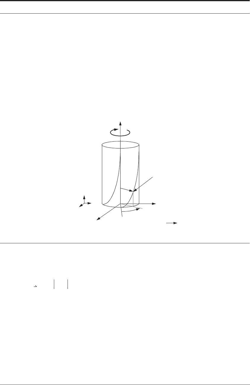
Figure 12.4 shows the geometry of a typical end mill with a right hand helix. The end mill is

modeled as a cylindrical surface of nominal radius R with N

helical cutting edges on its periph-

ery. The cutter is assumed to rotate and translate as shown in the figure. The final machined

surface, assumed to be generated by the combined effect of the two motions, is described by the

trochoidal path followed by the cutting edges.

FIGURE 12.4 Milling geometry in ideal case with no runout. The tool rotates around Z

perfectly aligned

with the machine tool Z

. Feed is then X and Y.

The position vector of a point P on the i

cutting edge is given by:

(12. 12)

where f is the cutter feed, θ

rot

is the rotation angle, λ is the helix angle, and

(12. 13)

The angle θ

is the circular pitch of cutter teeth and the angle u represents the phase difference

between the leading and trailing edges of the i

cutting edge due to the helix. The tooth path

segments at a particular cutter axial location are determined by the intersections between the tra-

jectories traced by successive teeth. The multiple intersections are found analytically from the

multiple values of θ

rot

at which the intersections occur:

Direction

of cutter

rotation

, X

Feed

direction

Point P

f θ

rot

2π

---------------- R

u+()cos+

⎩⎭

⎨⎬

⎧⎫

u+()sin{}j

λtan

-----------

⎩⎭

⎨⎬

⎧⎫

++=

rot

i 1–()θ

380 MODELING OF METAL CUTTING

(12. 14)

where n = 0, 1, 2, 3... represents the number of cutter revolutions.

The ideal three-dimensional milled surface can be generated using the equations above and

surface roughness parameters such as R

, R

, and R

max

can then be computed from the profile

data at any location along the cutter axis.

12.4.4 Roughness including runout

Eccentric motion of the cutter when mounted in the spindle can lead to runout - parallel axis

offset runout (PAOR) and axis tilt runout (ATR). In Figure 12.5, the parameters e and β repre-

sent the magnitude and direction, respectively, of the cutter axis offset. In Figure 12.6 axis tilt

runout is represented by τ (magnitude) and ρ (direction). To generate a 3-D map of the modeled

surface, the paths of discrete points, P

, along each flute of the cutter must be determined. The

cutter is divided into k discrete axial slices. For each slice, the position of the point P

is found as

the cutter is rotated through a complete revolution. This procedure is applied to each flute on the

cutter varying k over the entire axial cut. Each point P

is a position vector in an XYZ coordinate

system:

(12. 15)

where x

, y

, and z

are determined as:

(12. 16)

(12. 17)

(12. 18)

where θ

in the above expressions defines the angle from the X axis to each flute, i, at the free

end of the cutter:

(12. 19)

where i is varied from 0 to 3 for a cutter with four flutes. To determine the surface profile at

each axial depth k, successive tooth path intersection points are found. The 2-D profile is defined

rot

ui1–()θ

f θ

2nπ+()

4Rπ

-----------------------------

acos++=

i y

j z

k++=

fφ

2π

------ r

α–()cos εφβ+()cos l

–()τsin φρ+()cos+++=

α–()sin εφβ+()sin l

–()τsin φρ+()sin++=

1 αcos–()

λtan

---------------------------------------=

φ iθ

–=

MECHANISTIC MODELS 381

by the points that connect the intersections. The 2-D profile is determined for each axial slice,

then all slices are combined to form the 3-D surface map.

FIGURE 12.5 End milling with run out - top view

FIGURE 12.6 End milling with runout - side view (Figures 12.3 to 12.6 from Stori, King and Wright)

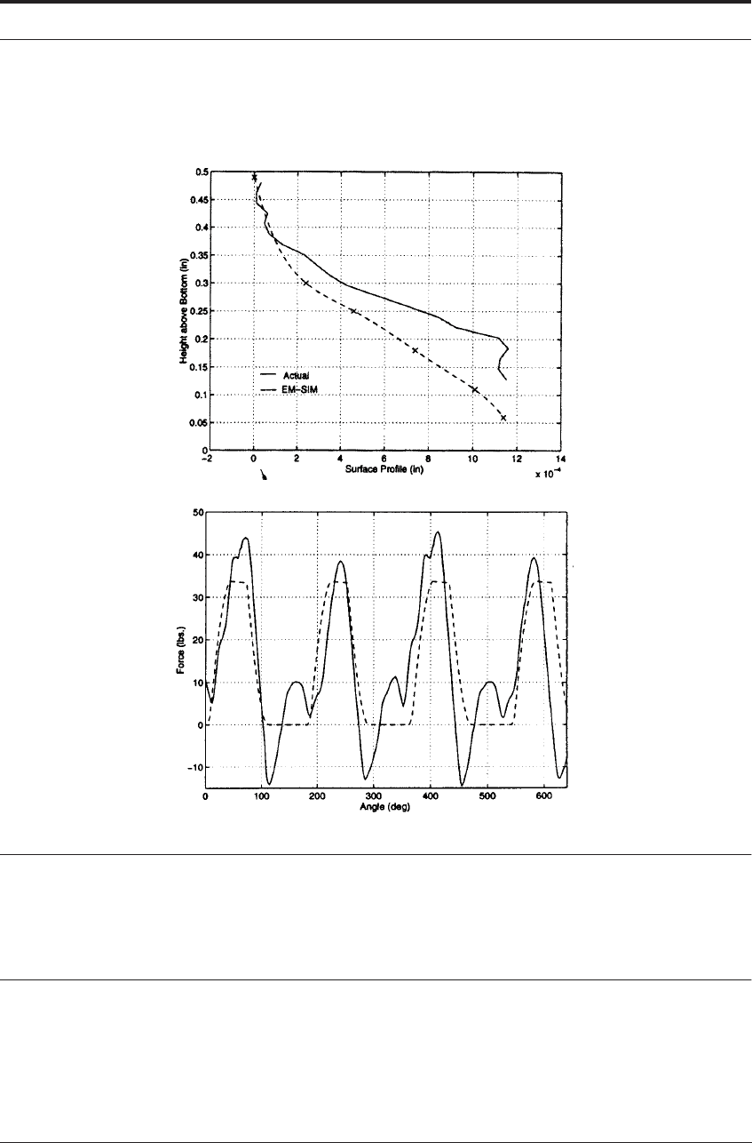
12.4.5 Case study: results from EMSIM

Figure 12.7a shows good agreement between EMSIM predictions and probing results for the

form-error on the walls of a pocket machined in 6061 aluminum with a 0.5 inch high speed steel

cutter.

Other results in the same set of experiments showed good agreement on forces (Figure

12.7b). Over time, these models are improving in their accuracy and scope, and can now be used

by practitioners to obtain higher accuracy in processes such as end milling. Knowing the pre-

dicted deflection in Figure 12.7a, allows the “roughing and finishing” sequence of the CNC

program to be closer to the “desired line” on the component being cut. However, the shape of

the contour will not change unless additional finishing passes are used to “trim out” the inside

i+1

i+2

i+3

ρφ

(

)

382 MODELING OF METAL CUTTING

corner of the pocket, where material might remain from a first finishing pass. This has to be done

with care to ensure that the pocket is not “overcut” at the top surface.

FIGURE 12.7 a) Contour plots showing the form error from equation 12.10. b) Comparisons between

experimental forces (solid lines) and predicted forces (dashed lines from EMSIM). Results of Mueller,

DeVor and Wright. Also see - http://madmax.me.berkeley.edu/webparam/demo2/summary2.html

12.5 FINITE ELEMENT ANALYSIS BASED MODELS

12.5.1 General introduction

For illustration purposes, Figure 5.7 is repeated below next to a finite element mesh (Figure

12.8). On the left, the classical equations developed in texts such as Carslaw and Jaeger

create

a continuum situation. By contrast, on the right, the finite element mesh, first used in this form

for metal cutting by Tay et al,

creates a discretized situation. Here, many small, interconnected