Smith G.T. Cutting Tool Technology: Industrial Handbook

Подождите немного. Документ загружается.

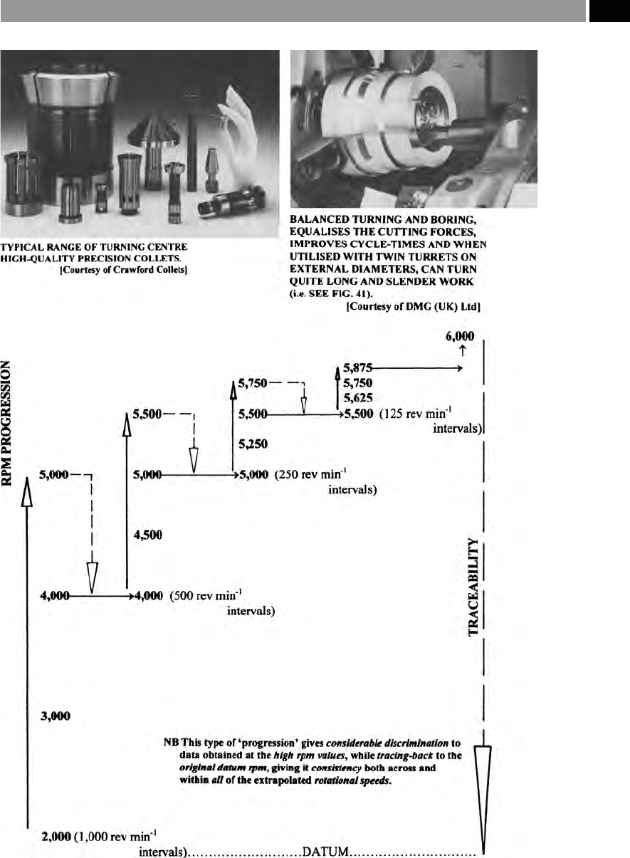
Figure 238. A ‘variable quasi-pilgrim stepped arithmetic progression’ – being utilised for UHSM (turning).

[Source: Smith, Littlefair, Wyatt & Berry, 2003]

Machining and Monitoring Strategies 483

situ. ese pre-shaped testpiece disks were: φ300 mm

by 6 mm thick, made from aluminium 2017F. e tool

with various cemented carbide tooling insert grades,

was held on a platform dynamometer (Kistler model:

9257B) – having complemntary charge ampliers

oupled to suitable data analysis soware. A range of

’s were utilised: 0.5, 1.0 and 1.5 mm, with a con-

stant and rapid feedrate of 30 m min

–1

. Apart from cut-

ting force analysis, turned surface texture, harmonic

roundness and micro-hardness results were obtained,

together with metallographical inspection of the sub-

surface regions. Hence, from this testpiece setup and

utilising the ‘progression’ for peripheral workpiece

speed strategy described above, the speeds ranged

from the conventional, through to UHSM.

UHSM: Turning Trends

Unlike the previous ndings of Youse and Ichida

(2000), where they suggested that the cutting forces

remained relatively constant across a broad spectrum

of UHSM – for turning operations. is UHSM turn-

ing work indicated that there was a decrease in mean

utting forces between 2,000 to 6,000 m min

–1

, with a

corresponding improvement in turned surface texture

(i.e. ‘Ra’) across this range. e harmonic departures-

from-roundness were inuenced by the sinusoidal ef-

fect of the uctuating tangential force as it progressed

around and along the turned surface’s periphery. is

harmonic behaviour was evident in the cutting force

data, where the analysis soware showed both a rising

and falling relationship, as the turning insert passed

over the rotating workpiece’s surface at great peripheral

speed. Such cutting force traces occur in high-speed

interpolation by the milling process, where there is a

general undulating increase/decrease in force genera-

tion, this being related to the axis transition cross-over

during cutter interpolation around the workpiece (i.e.

see Fig. 159). is cutting force undulation is the result

of the machine tool’s servo-motors reversing direc-

tion at these transitions, albeit, at signicantly slower

speeds than utilised for this UHSM turning work.

At such high turning speeds, chip-streaming was

pparent at peripheral speeds >4,000 m min

–1

. Chip-

streaming in UHSM by turning is the preferred chip-

form, as it exhausts the work-hardened swarf away

from the cutting vicinity, thereby minimising entan-

glement around the newly-formed turned workpiece

surface. At such high turning peripheral velocities,

the chip-streamed swarf is directed radially-away

from the work surface. Conversely, at lower rotational

workpiece-to-insert velocities, there was a marked

tendency for ‘chip-curling’. As a result of the inuence

of the insert’s geometry: nose radius and D

relation-

ship, the so-called ‘theta-eect’ in conjunction with the

feed-per-revolution occurs (i.e see Figs. 34c and d).

ere is a direct and predictable relationship to chip-

curl tendency when certain conditions arise at the

lower peripheral turning speeds, which is not apparent

at the UHSM turning range.

is UHSM turning applied research work, has

shown that it is feasible to employ ultra-fast turning

practices to the relevant components if the correct

tooling, workpiece and machine tool relationships can

be met.

9.6.3 Ultra-High Speed:

Trepanning Operations

Intoduction

Trepanning has been a well-recognised production

process for many years, it is principally utilised to pro-

duce large hole diameters, since this technique does

not require as much spindle power as solid drilling.

Moreover, in the ‘conventional’ approach to trepan-

ning, it is undertaken in one operation, but instead of

all the workpiece material being removed in the form of

a large volume of swarf, a cylindrically-shaped core is

le behind at the centre of the hole. us, this method

must be utilised for through-hole applications, assum-

ing that the internal feature – hole manufactured is the

scrap material. Conversely, in the UHSM trepanning

work shortly to be discussed, the two cutting edges are

externally set against the workpiece’s periphery, mak-

ing the ‘slug’ the product of the machining operations

(Fig. 239c).

UHSM – Trepanning Fix ture Design

As in the case of vertical turning, UHSM by trepan-

ning was undertaken on a vertical machining centre

utilising the same workholding arrangement (Fig.

239). Here, a special-purpose trepanning xture -

00 mm in overall length, was designed and manufac-

tured with twin-opposing tools (Fig. 239a). e tool-

ing was conventional TiN-coated cemented carbide

turning inserts – having straight toolholders these

being positioned on their sides in opposing directions

484 Chapter 9

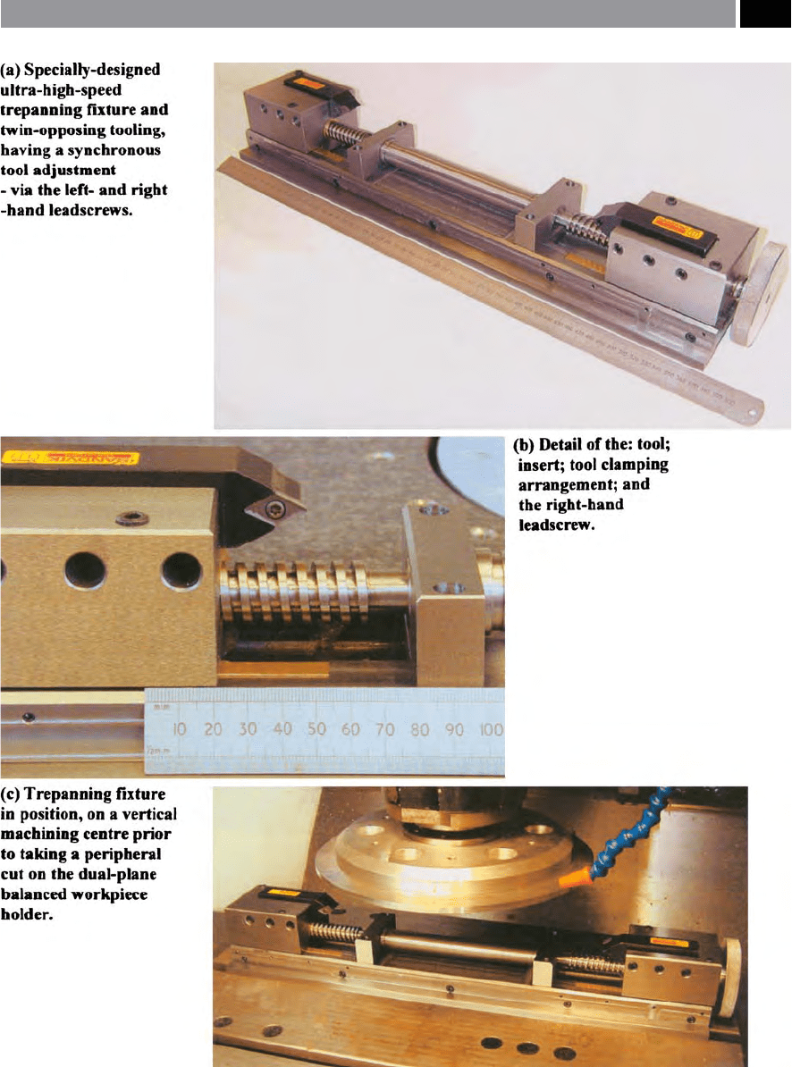
Figure 239. An ultra-high-speed trepanning xture and dual-plane balanced workpiece holder: utilised for an UHSM research

programme of work. [Source: Smith, Hills & Littlefair, 2005]

Machining and Monitoring Strategies 485

(Fig. 239b). So, by the simple action of turning a hand

wheel at its end, the tools could be simultaneously

opened and closed – for the required trepanned diam-

eter. is simultaneous tooling action was achieved,

by the singular rotating action of both the φ20mm by

4 m

m pitch le- and right-hand (i.e. M 20 × 4) square-

threaded leadscrews (Fig. 239c).

One of the major advantages of an UHSM trepan-

ning operation over its equivalent turning counterpart,

s that the cutting forces are virtually ‘cancelled-out’ , in

a similar fashion to a conventional ‘balanced turning’

peration (Figs. 41 and 238 – top right). Here in this

instance, one tool is set and positioned slightly ahead

of the other, thereby not only reducing the overall D

but allowing the ‘trailing tool edge’ to eectively act as

a ‘nishing tool’. is tooling positioning strategy pro-

duced an improved trepanned surface texture, while it

signicantly reduced the harmonic departures-from-

roundness, as metrologically assessed later on the

roundness testing machine. Moreover, by eectively

‘halving’ the D

, this allowed for an improvement in

the chip-streaming behaviour to be attained.

In a later modication to the trepanning xture (i.e.

not shown), a large micrometer drum with its inte-

grated vernier scale was tted in place of the knurled

adjustable hand-wheel (i.e see Fig. 239a), allowing for

some considerable discretion over the linear tooling’s

diametral adjustment. With such a large trepanning

xture – having the opposing tooling widely-spaced, it

is vital that these tools are centralised directly beneath

the machine’s spindle. Otherwise, there is a possibility

of both sine and cosine errors being present, creating

‘

Abbé-type errors’ , when adjusting and setting these

tools for their diametral in-feed.

UHSM – Trepanning Operation

is preliminary work on UHSM by trepanning, has

shown that with a suitably robust tooling xturing and

allowing a large (indirect) range of tooling diameter

adjustment – via the twin leadscrews, then not only is

the process feasible, but it oers considerably improved

machining performance and an inherent improvement

in trepanned surface and roundness characteristics,

over vertical turning processes. Possibly in a later

modication to a heavily-revised tooling adjustment

system, it might be possible to employ twin coaxial

ballscrews, with CNC servo-control, allowing auto-

matic control for machining tapers and proling to the

workpiece – by utilising the supplementary rotary axis

control in the machine’s CNC controller. Moreover,

one limitation to this UHSM trepanning technique is

the length of longitudinal cut that can be taken, prior

to the Z-axis motion causing the rotating part to foul

on the central portion of the trepanning xture. is

problem can be mitigated against, by increasing the

relative stand-o height of the twin-tooling from the

top of the xture by mounting each toolholder in an

extended tool block, so allowing greater Z-axis feeding

to be undertaken. Moreover by rearranging the tools

in relation to the workpiece, it would be possible to

‘turn’ shallow, depth internal trepanned features.

UHSM by trepanning oers signicant advantages

over ‘conventional’ vertical turning, in that, in this cur-

rent work, if was found that the trepanned workpiece

surface and roundness were signicantly improved

from the previously discussed UHSM by vertical turn-

ing, described in Section 9.6.2.

9.6.4 Artefact Stereometry:

for Dynamic Machine Tool

Comparative Assessments

Introduction

e use of machinable artefacts for the assessment of

machine tools such as machining centres, has been

utilised for some of years (i.e typically: NAS Stan-

dard 979: 1969; ISO Standard: 10791-7: 1997; Knapp,

1997), being developed just for this purpose. Both the

NAS and ISO Standard testpieces incorporated nota-

ble prismatic and rotational characteristics, manu-

factured to specic geometric and dimensional toler-

nces, such as: at the top, an φ110 mm circular feature;

6 mm below this round shape, an 110 mm diagonal

feature is cut; a central φ30 mm though-running hole

is produced; with a series of counter-bored holes at

four equi-spaced quadrants are generated these be-

ng situated 6 mm below the diagonal shape. Taken in

cross-section, the geometry of the machinable arte-

facts resembles a stepped component, having an over-

ll height of 50 mm. In fact, this type of artefact has

long been employed by industry to establish the over-

all machining performance capabilities of a particu-

lar machine tool under test. However, although this

prismatic and rotational featured machinable artefact

achieves some measure of conformance and indicates

the likely operational performance of the machine

tool, it does tend to have several signicant limita-

tions, such as the:

•

Overall dimensional size of the artefact is quite

small – when compared to that of the volumetric

envelope of typical industrial machining centres,

486 Chapter 9

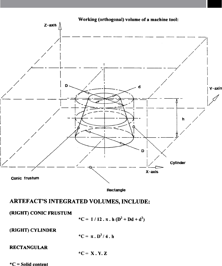
Figure 240. Artefact stereometry, illustrating its integrated volume geometries, for a:

1. (right) conic frustum,

2. (right) cylinder,

3. rectangular volume of machine tool’s axes.

[Source: Smith, Sims, Hope & Gull, 2001]

Machining and Monitoring Strategies 487

•

Circular feature cannot be directly compared to

that of diagnostic instrumentation – such as the

Ballbar, as the diameter of this rotational feature

diers from that of the standard Ballbar sizes,

•

Weight of the artefact does not realistically com-

pare to any workspaces normally placed on the ma-

hine tool in its ‘loaded-state’ , meaning that ‘true’

machine tool loading-conditions are not directly

comparable.

With these machinable testpiece limitations in mind,

it was thought worthwhile developing a new calibra-

tion strategy for such machine tools, but here, under

ore realistic ‘loaded conditions’ , also this new arte-

fact being more directly comparable to diagnostic

instrumentation (i.e. such as the Ballbar), but having

considerably larger volumetric size and weight, with

the capacity for reuse of the expensively-produced

precision part of the machinable artefact’s assembly.

Stereometric Artefact – Conceptual Design

Stereometry has been a concept that has oen been

over-looked, but it deals with the volumetric content of

a range of geometric shapes. However, if this ‘volumet-

ric concept’ is carefully integrated into a single artefact,

it could be employed for calibration work on machine

tools such as machining centres (i.e see Fig. 240). Here,

the cylinder was represented by three machinable aero-

space aluminium disks (grade: 2017F – produced from

6 m

m sheet, to nominally slightly >φ3

00 mm) each one

being set 100 mm apart in height (i.e. disks: 1, 2 and 3)

and aer machining, the disks were exactly φ3

00 mm

(i.e see Fig. 241). e conic frustum included angle

was 22.5°, this being the result of producing 4 equi-

spaced holes in each disk. Starting on the bottom (disk

1), then stopping the machine and tting the middle

disk (disk 2) and drilling the 4 holes and likewise up-

ard to the top disk (disk 3), while simultaneously

producing a 3-dimensional Isosceles triangle

(Fig.

241). Each disk had these individual holes being set

at an angular relationship of 90° equi-spaced apart, so,

hen they are taken as a ‘volume’ , a conic frustum is

produced (Fig. 242b). ese geometric and volumet-

33 ‘Isosceles triangle’ , has two sides with two angles being equal,

but in this case, with the geometry of a right-angled triangle.

NB ese side lengths and associated angles can be varied,

so long as they both (i.e lengths, or angles) remain of identical

proportions.

ric relationships were intrinsically set and datumed to

a centrally-machined slot in the base of the precision

mandrel. is fact, meant that the exact angular and

volumetric relationships remained in-situ, when the

stereometric artefact was then taken o the machine

tool for subsequent analyses.

Stereometric Artefact – Machining Trials

Prior to the stereometric artefact having its machin-

able disks milled, the initial test machine tool (i.e. in

the initial trials on a Cincinnati Milacron Sabre 500

equipped with a Fanuc OM CNC controller) was fully

diagnostically calibrated by: Laser interferometry;

long-term dynamic thermal monitioring of its duty-

cycles in both a loaded and unloaded condition; to-

gether with Ballbar assessment. Prior to discussing

the actual machining of the disks, it is worth taking a

few moments to consider the precision mandrel that

accurately and precisely locates each disk in the de-

sired orientation, with respect to each other and the

machine tool’s axes. is mandrel body was produced

from a eutectic steel

(0.83% carbon), which aer

through-hardening to 54 HR

, was precision cylindri-

34 ‘Eutectic steel’ or ‘Silver-steel’ as it is generally known, due to

its almost ‘shiny appearance’ when compared to other grades

of plain carbon steels. In brief, this 0.83% carbon content steel

is so-called a eutectic* steel as it relates to the eutectic com-

position derived from the iron-carbon thermal equilibrium

diagram. Producing an 100% pearlitic structure (i.e. hence its

‘metallographic-brilliance’ , or its ‘irridescence’) when viewed

under a microscope, exhibiting ne alternate layers of: Fe

and Fe. To harden eutectic steel, its temperature is raised

slightly above the ‘arrest point’ (i.e. arrest point here, equals

723°C, so hardening could be undertaken at ≈765°C) into

‘γ-solid solution’ (i.e. austenitic region), then rapidly quenched

and agitated in water to prevent carbon atomic diusion (i.e

undertaken at greater than the ‘critical cooling velocity’), with

the carbon atoms now being eectively ‘xed’ – though not

intrinsically part – of the atomic lattice structure. is carbon

entrapment, creates intense local strains that block dislocation

movement. Hence, the resulting structure is both hard and ex-

tremely strong, but also very brittle. Microscopically, the hard-

ened structure appears as an array of random needles, being

completely dierent from the original pearlitic structure. is

needle-like structure formed by trapped carbon atoms in an

iron crystal lattice is termed, ‘martensite’. us, the degree of

hardness – aer quenching, being proportional to its lattice

strain. Aer hardening, the mandrel needed to be tempered.

Tempering is a controlled heat-treatment process to allow

some of the trapped carbon to escape from the interstitial

spaces between the iron atoms distorted lattice structure,

where they eventually form particles of cementite.

488 Chapter 9

cally-ground on the three register diameters, with the

top and bottom faces being surface ground. Previous to

this heat-treatment and the grinding processes, dow-

elling datums (i.e. φ6 m

m) were drilled and reamed,

then 3 equi-spaced tapped clamping holes were pro-

duced for each disk, along with a ground tenon groove

in the base – all these features being orientated to the

geometry of the machines axes (Fig. 241).

Several unique features are introduced within the

machinable portions of the disks, such as:

•

ese aerospace-grade aluminium disks were

milled to φ3

00 mm diameter, which directly cor-

responded to the radial path of the Ballbar (i.e see

Fig. 242a) – used previously for diagnostic machine

tool assessment, ensuring that some degree of cor-

relation occurred between them,

•

e three Z-plane disk heights of: 70, 170 and

270 mm (i.e. modied from the original design Fig.

241), coincided with both the X-Y plane table po-

sition and vertical heights utilised for the Ballbar

plots, creating a reasonably large cylindrical volu-

metric envelope (Fig. 242b). Moreover, the stereo-

metric artefact was both designed and orientated to

coincide with the start and nish positions of the

Ballbar’s polar traces,

•

e 4 circular interpolated holes (φ10 mm) on each

disk (i.e see Fig. 241), were geometrically posi-

tioned to form a three-dimensional Isosceles tri-

angle at the three Z-axis heights for each quadrant

of these disks – with the 1

an 3

holes relating to

the axes transition points in the X-Y planes. us,

each of the interpolated milled holes in the face of

separate disk’s, produced the geometric stereom-

etry of a conic frustum, having an included angle of

22.5° – when the angular orientation of the middle

disk is ‘soware-realigned’ to produce a straight-

line relationship (i.e see Fig. 242b),

NB e temperature at which tempering is undertaken is

critical, thus between 200–300°C, atomic diusion rates are

slow with only a small amount of carbon being released,

thereby the component retains most of the hardness. So if

higher ‘soaking-temperatures’ are employed (i.e between

300–500°C), then this creates greater carbon diusion form-

ing cementite, with a corresponding drop in the component’s

bulk hardness.

* A eutectic structure is a two-phase microstructure resulting

from the solidication of a liquid having the eutectic compo-

sition: the phases exist as ne lamellae that alternate with one

another. (Sources: elning, 1981, Alexander et al., 1985; Cal-

lister, Jr. et al., 2003)

•

Overall weight of the mandrel and three disk as-

sembly was 38 kg, consequently, this could be

considered as a realistic ‘loaded condition’ for the

machine tool to operate under, from a practical

sense.

In order to minimise the milling forces on the ma-

chinable disks, HSM was employed using a spindle-

mounted ‘Speed-increaser’

(Fig. 243a) equipped with

a φ6 m

m slot drill. e HSM speed-increaser was oper-

ated under the following conditions: 18,000 rev min

–1

;

at a circular interpolation feed of 750 mm min

–1

; with

the disks having 1 mm of excess stock for each ma-

chinable disk – to be milled by circular interpolation.

In Fig. 243a, the last machinable disk has been located

and clamped and the whole mandrel-and-disk assem-

bly was nearing completion, having previously had its

φ1

0 mm quadrant-positioned holes for each disk ma-

chined by small circular interpolated motions by the

slot drill (i.e. see the sectional details of the φ1

0 mm

hole geometry in each disk’s quadrant co-ordinates, as

illustrated in Fig. 241).

Stereometric Artefact – HSM Results

Aer HSM by milled interpolation on the vertical

machining centre, the complete artefact with its ma-

chinable disks in-situ, was carefully removed from

the machine tool, then automatically-inspected for

its quadrant hole positions and disk diameters, on an

Eastman bridge-type Co-ordinate Measuring Machine

(CMM). is CMM having previously been thermally

error-mapped, then checked with a ‘Machine Check-

ng Gauge’

(MCG) – prior to artefact inspection.

e CMM utilised a specially-made and calibrated

35 ‘Speed-increasers’ , are a means of multiplying the rotational

speed of the machine’s spindle, by utilising a xed relationship

geared head. Here, this actual speed-increaser had a 3:1 gear-

ing ratio, equating to a top speed of 18,000 rev min

–1

, when it

is operating at the top speed for this particular machine tool

(i.e. 6,000 rev min

–1

NB Normally, these HSM milling/drilling geared heads are

limited to a certain proportion of running time per hour at

its top speed, as they could over-heat and thereby damage the

bearing/gearing mechanism.

36 ‘Machine Checking Gauge’ (MCG), is utilised to check a

CMM’s repeatability and accuracy and to detect for any po-

tential ‘lobing-type errors’ from the ‘triggering-positioning’

mechanism of the touch-trigger probe, these being invariably

used on such machines.

Machining and Monitoring Strategies 489

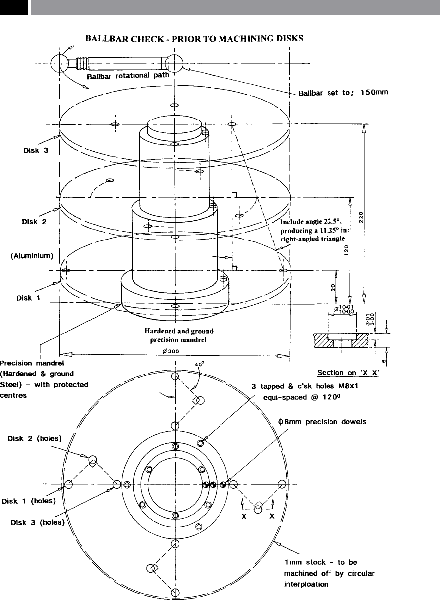
Figure 241. Artefact stereometry was designed for the volumetric and positional uncertainites on machining

centres, by: HSM interpolation of machinable disks. [Source: Smith, Sims, Hope & Gull, 2001]

490 Chapter 9

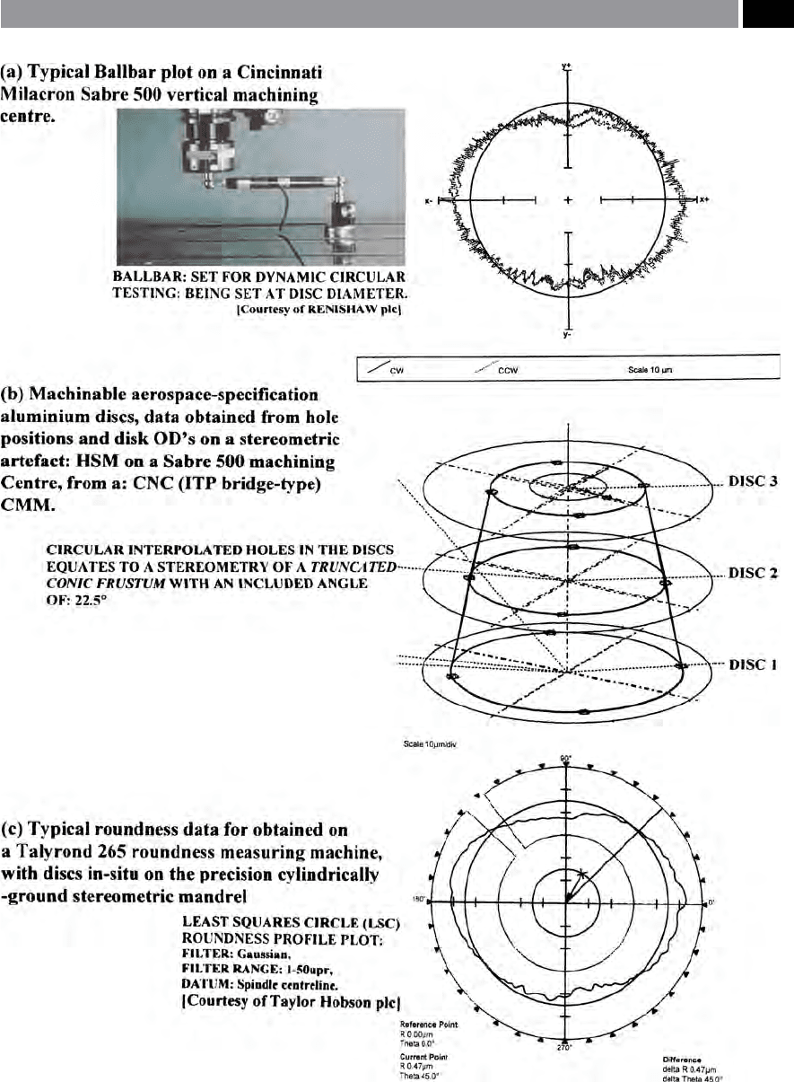
Figure 242. HSM (milling) of three machinable disks in-situ on a stereometric artefact, on a vertical machining centre. [Source:

Smith, Sims, Hope & Gull, 2001]

Machining and Monitoring Strategies 491

cranked-probe – with its calibration obtained from

the ‘reference measurement sphere’ being located on

the CMM’s table, utilised to inspect the φ1

0 mm hole

geometry and there respective co-ordinate positions.

is probe arrangement was swapped for a conven-

tional ‘touch-trigger probe assembly’ to measure the

machinable disk diameters – while holding the same

cartesian co-ordinate relationships as when it was

riginally UHM. Later – without ‘breaking-down’ ,

while still maintaining the same angular orientation,

this stereometric artefact assembly was inspected on a

roundness testing machine (Taylor Hobson: ‘Talyrond

265’) for individual disk parameters of roundness and

cylindricity

assessment – for the ‘three-disk relation-

ship’. e results of all of these ‘averaged’ roundness

measurements and Ballbar polar plots are graphically

depicted as histograms in Fig. 243c.

When a comparison is made of these results from

three individual and completely diering inspec-

tion procedures, namely: Ballbar; CMM; and Taly-

rond, they show some degree of measurement con-

sistency individually, but less so when each disk data

is grouped. For example, in the case of the Ballbar, it

ndicated a 1 µm variation (i.e. range) from the top-to-

bottom disks, while having a mean value of 17.5 µm.

e Talyrond polar plots (i.e. ‘Least Squares Reference

ircle’

: departures from roundness) also produced

consistent roundness results, ranging from <4 µm,

having a mean value of ≈14 µm. Conversely, the larg-

est variability occurred with the CMM, producing a

37 ‘Cylindricity’ , can be dened as: ‘e minimum radial separation

of 2 cylinders, coaxial with the tted reference axis, which totally

enclose the measured data’. (Source: Taylor Hobson, 2003)

NB A ‘working denition for cylindricity’ , might be: ‘If a

perfectly at plate is inclined at a shallow angle and a parallel

cylindrical component is rolled down this plate. If it is a truly

round cylinder then as the component rolls, there should be

no discernible radial/longitudinal motion apparent’. (Sources:

Dagnall, 1996; Smith, 2002)

38 ‘Least Squares Reference Circle’ (LSC1), can be dened as: ‘A

line, or gure tted to any data such that the sum of the squares

of the departure of the data from that line, or gure is a mini-

mum’. is is also the line that divides the prole into equal

minimum areas

NB 

is LSC1 is the most commonly used ‘Reference Circle’.

e ‘out-of-roundness’ , or ‘departures-from-roundness’ as it

is now known, is then expressed in terms of the maximum

departure of the prole from the LSC1 (i.e. the highest peak

to lowest valley – on the ‘polar plot’). (Source: Taylor Hobson,

2003)

range of 15 µm, with a mean value of ≈23 µm. Prior to

discussing why the CMM results signicantly varied

from those obtained by both the Ballbar and Talyrond,

it is worth visually looking at a comparison between

the general proled shapes of typical ‘polar plots’ pro-

duced by both these techniques. In Fig. 242a, a rep-

resentative ‘polar plot’ from a Ballbar is shown and,

likewise in Fig. 242c, one from a Talyrond is depicted.

eir respective proled shape geometry in terms of

harmonics, is remarkably alike, illustrating the same

generally similar lobed-shape combined with its iden-

tical angular orientation.

Returning to the CMM results, only a few data

points are utilised to obtain a measured diameter,

while with the Ballbar and Talyrond alike, they liter-

ally take thousands of data points to obtain the polar

plotted proles. If, when the CMM touches each of

the machinable disk’s prole with the ‘touch-trigger

robe’ , this co-ordinate’s data could have been ob-

tained at the extremes of the elliptical shape, namely,

at its major and minor diameters, this may account for

such a variation in both the range and discrepancies,

when compared to the data obtained by the Ballbar

and Talyrond.

e four φ1

0 mm holes in each disk that were pro-

duced by HSM utilising circular interpolation at their

respective quadrant positions (Figs. 241 and 242b), are

given in the form of tabulated data in Table 16 – in

terms of their positional accuracy and radial change,

from their theoretical centres. From this φ1

0 mm hole

data, then the radial change for each disk, from the

op, middle and bottom disks, was: 46 µm: 45 µm: and

42 µm: respectively, giving a positional uncertainty

across these disks of 4 µm.

Conversely, if the dierence is considered for the

three stacked disks with respect to their angular rela-

tionships to each other, at: 0°; 90°; 180°; 270°; then their

ngular positional changes are: 46 µm; 26 µm; 32 µm;

and 49 µm; giving a positional uncertainty of 23 µm.

is positional uncertainty is still relatively small con-

sidering that in this case, each hole’s position is on a

dierent Z-axis plane – spanning 200mm in height.

Although if one considers the ‘Grand mean’ for both

cases then they have a positional uncertainty of just

1 µ

m, which for a machine tool that at this time was

around three years old is quite exceptional – having by

now, undertaken considerable industrial machinabil-

ity trials for the automotive and aerospace industries,

but admittedly, this vertical machining centre had pre-

viously been both Laser- and Ballbar-diagnostically

corrected – showing the ‘true’ relevance of calibration

to resolve and reduce any ‘errors’!

492 Chapter 9