Skiadas C.H., Skiadas C. Chaotic Modelling and Simulation. Analysis of Chaotic Models, Attractors and Forms

Подождите немного. Документ загружается.

104 Chaotic Modelling and Simulation

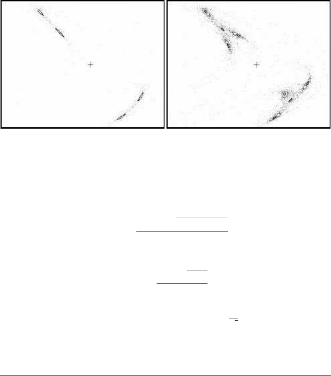
(a) a = 1.02 (b) a = 1.3

FIGURE 5.4: Higher-order bifurcations in the cosine H

enon model

This system has ﬁxed points at

x = y =

b − 1 ±

(

b − 1

)

+ 4a

When b = −1, these ﬁxed points become:

x = y =

−1 ±

√

1 + a

which is precisely the same as the ﬁxed points for (5.2).

Similarly, when b = 1, the provided value is x = y = ±

√

which is also the same

value as that provided from the diﬀerence equation case.

5.5 Variants of the H´enon Delay Diﬀerence Equation

A number of variants of the H

enon model give rise to some interesting attractors.

We discuss a couple of these variants, involving either higher-order delays (sections

5.5.1, 5.5.2), or simply changes in the way the ﬁrst-order terms are introduced (sec-

tions 5.5.3, 5.5.4).

5.5.1 The third-order delay model

An extension to higher delay dimensions is given by

t+1

= bx

t−3

+ ax

(1 − x

) (5.8)

The H´enon Model 105

Similar to (5.2), the diﬀerence delay equation (5.8) can be turned into a system of

four ordinary diﬀerence equations. The number of time delays in the delay diﬀerence

equation is equal to the number of new equations of the ordinary diﬀerence equation

system. The model (5.8) exhibits three time-delay periods, and is characterised by a

very interesting attractor when the parameters are a = 3.2 and b = 0.2 (Figure 5.5).

FIGURE 5.5: A third-order delay model

5.5.2 Second-order delay models

The following variant, with a second-order delay term, is extremely simple, having

only one parameter b:

t+1

= −bx

+ x

t−2

(5.9)

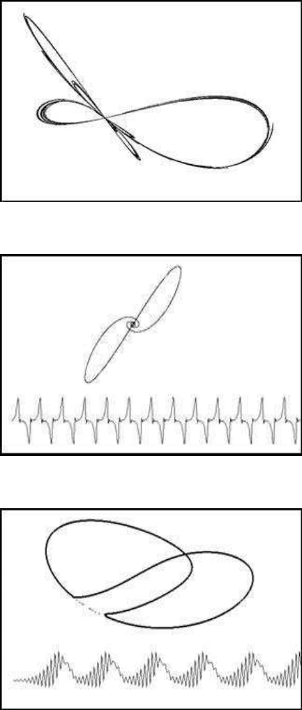
The attractors of the model are however very interesting. Figure 5.6 for instance

shows the attractor when b = 1.37.

Another interesting variant with a second-order delay is the following:

t+1

= x

+ a(x

t−2

− x

t−2

) (5.10)

When a = 0.52, the resulting map and the related oscillations (t, x) are illustrated in

Figure 5.7.

A more complicated model is given by:

t+1

= bx

t−1

− ax

+ x

t−2

(5.11)

This is a two-parameter delay model with both ﬁrst- and second-order delay terms.

There is a characteristic limit cycle obtained when the parameters have values a =

1.2 and b = 0.75. The repeated oscillations and the limit cycle are presented in

Figure 5.8.

106 Chaotic Modelling and Simulation

FIGURE 5.6: A second-order delay model

FIGURE 5.7: The order-2 delay model

FIGURE 5.8: A complicated delay model

The H´enon Model 107

5.5.3 First-order delay variants

Interesting ﬁrst-order delay variants of the H

enon model arise when one of the two

terms on the right-hand side of (5.1) is altered.

For example, if we replace the quadratic term with a delay logistic term, the re-

sulting model has the form:

t+1

= bx

t−1

+ ax

(1 − x

t−1

) (5.12)

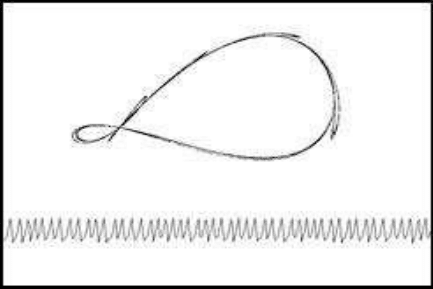
Figure 5.9 illustrates the two-dimensional map, and the related oscillations, when

a = 2.35 and b = 0.2.

FIGURE 5.9: A H

enon model with a logistic delay term

Another variant arises by altering the ﬁrst term:

t+1

= bx

t−1

+ 1 − ax

(5.13)

For a = 1.72 and b = 0.6, the resulting map and related oscillations are illustrated in

Figure 5.10.

As in the case of the original H

enon model, it is more convenient, for further

analysis, to transform (5.13) into a system of two diﬀerence equations:

t+1

= x

+ 1 − ax

t+1

= bx

(5.14)

The Jacobian determinant of (5.14) is

det J = −bx

This indicates that the model (5.14) has properties diﬀerent from those of the H

enon

model.

108 Chaotic Modelling and Simulation

FIGURE 5.10: A variation of the H

enon model

5.5.4 Exponential variants

The introduction of an exponential term into (4.20) gives rise to a variant with a

very complex attractor (Figure 5.11, a = 0.8, b = 0.36), which we will call the Henia

attractor. The equation is

t+1

= bx

t−1

+ 1 − ax

−ax

t−1

(5.15)

FIGURE 5.11: An exponential variant of the H

enon model

The H´enon Model 109

5.6 Variants of the H´enon System Equations

Other interesting variants arise from altering the system (5.2). An example is the

following:

t+1

= bx

+ cy

− 2x

t+1

= a(y

− x

)

(5.16)

For appropriate values of the parameters, interesting stone-shaped attractors appear

(Figure 5.12 (a = 0.8, b = 0.48, c = 1.1)).

FIGURE 5.12: A 2-diﬀerence equations system

Another set of extensions involves the introduction of a third variable:

t+1

= bx

− y

− x

t+1

= −cz

+ x

t+1

= a(z

− x

)

(5.17)

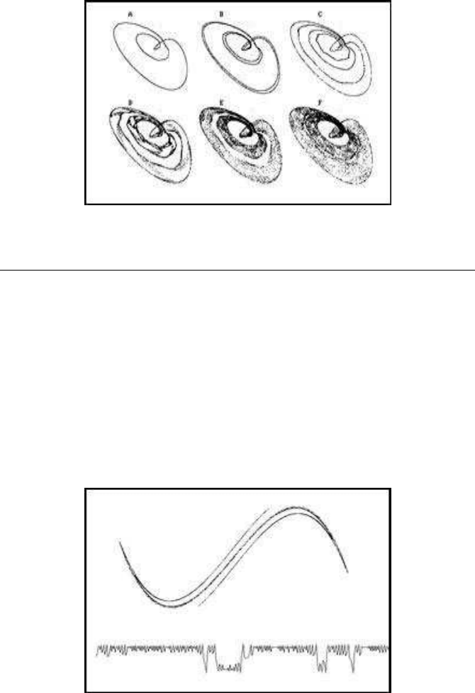
Depending on the values of the three parameters, this model exhibits limit cycles,

bifurcation and ﬁnally chaotic behaviour. Figure 5.13 illustrates these cases. The

parameters a and c are ﬁxed at 0.95 and 0.4 respectively, while b takes the values

0.62, 0.628, 0.6337, 0.6348, 0.6355 and 0.637 respectively. The graphs represent the

(x, y) map.

110 Chaotic Modelling and Simulation

FIGURE 5.13: A three-dimensional model

5.7 The Holmes and Sine Delay Models

5.7.1 The Holmes model

The Holmes model can be thought of as an extension of the H

enon model (Holmes,

1979a). The general form of the Holmes model is:

t+1

= bx

t−1

+ ax

− x

The Holmes model, when b = −0.2 and a = 2.765, provides a characteristic sigmoid

map and quite complicated chaotic oscillations (Figure 5.14). When b > 0, the

FIGURE 5.14: The Holmes model (a = 2.765, b = −0.2)

Holmes model gives a rich sigmoid form (Figure 5.15, b = 0.3 and a = 2.4).

The H´enon Model 111

FIGURE 5.15: The Holmes model (a = 2.4, b = 0.3)

5.7.2 The sine delay model

The model proposed by Holmes is an approximation

of a sinusoidal one, called

the sine delay model, of the form:

t+1

= bx

t−1

+ a sin(x

) (5.18)

This model, for relatively small values of a, shows similar behaviour to that of the

Holmes model. However, when a takes large values, the map changes into a series

of sigmoid forms. The number of maxima or minima of the resulting curves can be

estimated according to the number of solutions of the equation

(1 − b)x − a sin(x) = 0.

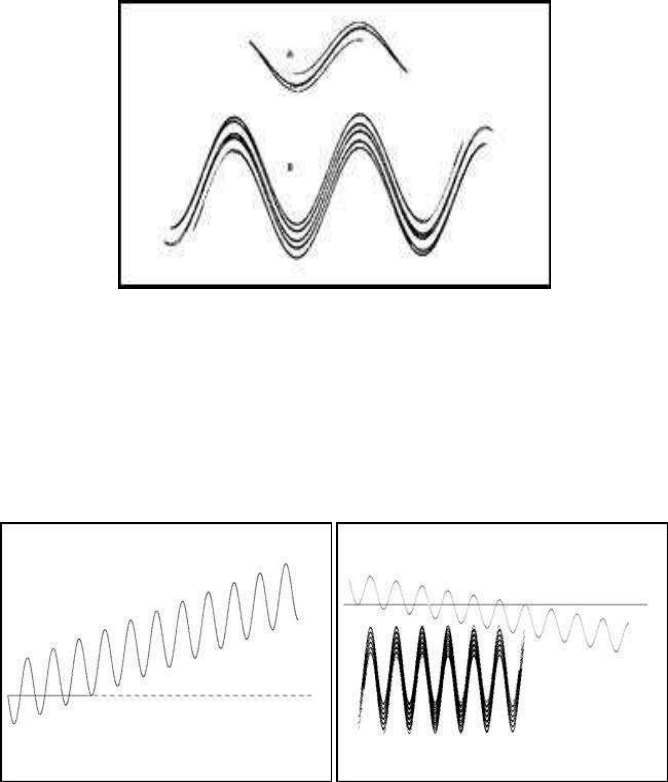
In the example presented in Figure 5.16, the delay parameter is ﬁxed at b = 0.3 in

both cases, and the parameter a is set to a = 3.0772 for the case A and a = 2 ×3.0772

for the case B. It is clear, by observing the resulting maps, that by doubling the value

of a, the number of maxima or minima is also doubled.

When b is small, there is a close relation between the maxima and minima of this

map, and the maxima and minima of the function

y = f (x) = (1 − b)x − a sin(x).

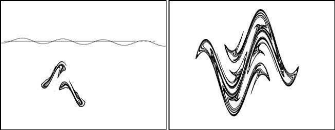
The relation can be seen in Figure 5.17(a). Note further that the range of x values for

the map ends exactly at the last solution to f (x ) (the solutions to f (x) = 0 are exactly

the ﬁxed points of the sine delay map). Figure 5.17(b) shows the case where b = 0.3

and a = 6.5(1 −b)π.

When b takes values closer to 1, say b = 0.88, the situation changes radically, as

the attractor is now separated in two very similar parts (Figure 5.18(a)). There is now

The approximation can be seen by replacing sin(x) with its third degree Taylor approximation, x −

112 Chaotic Modelling and Simulation

FIGURE 5.16: The sine delay map (b = 0.3)

(a) Solutions to the ﬁxed point equation for

the sine delay model

(b) Maxima and minima of the sine de-

lay model and the corresponding ﬁxed point

equation

FIGURE 5.17: The sine delay model

The H´enon Model 113

little relation with the maxima and minima of the ﬁxed point equation. The values

a = 3 and b = 0.8 produce the very interesting attractor of Figure 5.18(b).

(a) b = 0.88 (b) a = 3, b = 0.8

FIGURE 5.18: The sine delay model for large b

Things change quite a bit when b = 1. In this case, the map takes the form

t+1

= x

t−1

+ a sin(x

The resulting simulation is shown in Figure 5.19(a) for a = 1.2. The process follows

a random sequence that gradually occupies the entire (x

t−1

, x

) plane. The basic

forms of the two generating shapes can be seen more clearly in Figure 5.19(b), where

a = 0.8.

Both shapes are identical but they are a ninety-degrees rotation of each other. Both

shapes become closer to a square with rounded corners as the parameter a takes very

small positive values (Figure 5.20,a = 0.1).