Skiadas C.H., Skiadas C. Chaotic Modelling and Simulation. Analysis of Chaotic Models, Attractors and Forms

Подождите немного. Документ загружается.

84 Chaotic Modelling and Simulation

lations appear very naturally in a system with memory. This is because the model ex-

pressing the behaviour of the system integrates into the diﬀerential-diﬀerence equa-

tions the past as one or more delay variables. As a consequence, delay means oscil-

lations.

Experience conﬁrms the appearance of oscillations in very many systems where

delays are inherent. Delays in human decisions on social, economic, technolog-

ical or political systems may lead to oscillations. Short- or long-term economic

cycles, social or political changes, innovation or technological cycles may be ex-

pected when time delays are present. Biological cycles, biological clocks and other

oscillating mechanisms of humans and other living organisms are some of the nu-

merous cases where delays are present in nature. Chemical oscillations and the

Belousov-Zabontiski reactions modelled and studied extensively by Prigogine and

his co-workers (Prigogine and Lefever, 1968; Prigogine et al., 1969; Nicolis and

Prigogine, 1981; Prigogine, 1995, 1996, 1997) are also examples of the eﬀect of de-

lays in the formation of the intermediate substrates until the formation of the ﬁnal

product.

4.4 A More Complicated Delay Model

Using the same method presented above, we simulate a more complicated delay

model, which has a more stable oscillating behaviour. The general delay equation

for this model is

˙x = −ax

t−1



1 − x



(4.8)

The oscillations of (4.8) are quite stable when a >

, and they exhibit a very inter-

esting behaviour for some values of a. The parameter b is an integer, and two distinct

cases are considered, depending on the parity of b. When b = 1, the model (4.8) re-

duces to a continuous delay logistic model.

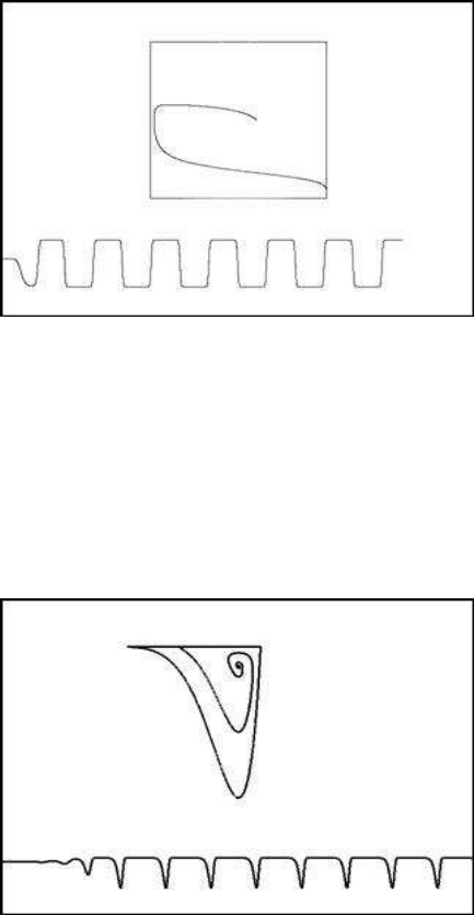
Of special importance is the case where b = 2. When b = 2 and a = 14, sim-

ulation results in the very important form shown in Figure 4.6. The resulting two-

dimensional map is an almost perfect square, irrespective of the starting point, as

long as this point is inside the square, i.e. if the starting values are in [0, 1]. This

rectangular form shows for any a >

, with the sharpness of the corners depending

on the value of a. In the case studied in Figure 4.6, the linear spline approximation

method was used with n = 30, h = 0.001 and initial value x = 0.2, and it gave

very good results. The rectangular oscillations appear to be quite perfect and may be

useful in several applications.

The oscillations are quite diﬀerent when b is odd. The behaviour in this case is

similar to that of the discrete delay logistic model (Figure 4.7, b = 1, a = 3.7,

n = 15). The delay equation in this case is:

˙x = −ax

t−1

(1 − x

) (4.9)

The Delay Logistic Model 85

FIGURE 4.6: Delay model (b = 2); a square pattern

FIGURE 4.7: Delay logistic model

86 Chaotic Modelling and Simulation

4.5 A Delay Diﬀerential Logistic Analogue

The appropriate diﬀerential equation analogue to the delay diﬀerence equation (4.9)

is:

˙x

= bx(1 − x

) (4.10)

In order to perform a simulation of (4.10), the method of linear spline approxima-

tion presented in page 83 will be used. The intermediate step is s and the iteration

step is d. The delay term is included only in the ﬁrst equation. It is the last term to

the right of the ﬁrst equation. By changing this delay term, or replacing it by another,

many interesting cases arise.

= x

+ bx

(1 − x

= x

−

− x

= x

−

− x

m−1

(4.11)

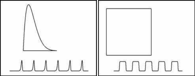
Figure 4.8(a) illustrates the (x

, x

m+1

) and (t, x

) diagrams for the case where b =

1.22, d = 0.01, s = 3 and m = 14. There is a clear similarity with the previous case

of the diﬀerence equation above.

The simulation producing Figure 4.8(b) is based on another delay equation:

˙x

= bx

(1 − x

) (4.12)

The parameters in Figure 4.8(b) are m = 15, s = 6, d = 0.001 and b = 2.6. As

can be seen from the ﬁgure, the (x

, x

m+1

) graph is an almost perfect square. Close

inspection, however, will show that the corners are not very sharp. This is due to the

choice of the parameters and of the integration step. Nevertheless, equation (4.12) is

a continuous equation very appropriate for expressing a square. The oscillation turns

out to exhibit a step form.

In both cases presented above, b was selected close to its upper limit. However,

one can have several intermediate cases of particular interest.

4.6 Other Delay Logistic Models

Another form of a delay logistic model is expressed by the following diﬀerence

equation:

t+1

= ax

+ bx

t−m

(1 − x

t−m

) (4.13)

The Delay Logistic Model 87

(a) Delay Logistic (m = 14) (b) An almost perfect square

FIGURE 4.8: Oscillations and limit cycles in delay logistic models

This is a delay model that integrates the inﬂuence of a logistic like interaction to

the future. As a simple example, consider the impact of a “word-of-mouth” com-

munication between x adopters and (1 − x) potential adopters of an innovation or an

idea, communicated m time units in the past, and inﬂuencing people at the present

time. This happens very frequently in marketing, economic, social or political sys-

tems. The impact of this time-delayed inﬂuence to the evolution of x in the future

will be studied by varying the width of the delay interval m and the values of the

parameters a and b. The ax

term represents the current adopters who continue, and

the bx

t−m

(1 − x

t−m

) term represents the new adopters.

In this model, limit cycles, bifurcation and chaotic behaviour appear. A large

variety of oscillations and chaotic oscillations appear, depending on the level of the

delay. But, even in the simplest cases of one or two units of delay, the behaviour of

the system is quite complicated. High delay levels ensure chaotic behaviour.

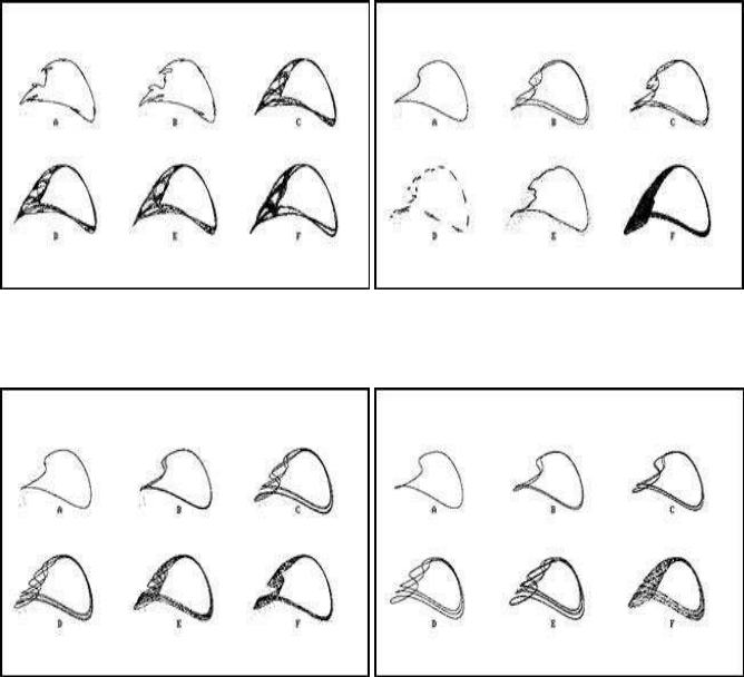
The simplest form of (4.13) is when m = 1. The more interesting forms appear in

Figure 4.9(a). The six realisations, A through F, illustrate the behaviour of the system

when b is 1.706, 1.717, 1.751, 1.758, 1.77 and 1.795 respectively. Throughout, a was

set to 0.9 and x

was set to 0.1. As b increases, limit cycles are followed by chaotic

behaviour.

Figure 4.9(b) examines the case where m = 2. Again, limit cycles, bifurcation

and then chaos appear as b increases. ﬁgures A through F correspond to b values of

1.2, 1.22, 1.241, 1.252, 1.259 and 1.269 respectively (a = 0.9 and x

= 0.1).

The m = 3 time delay has an interesting eﬀect on the two-dimensional graph (Fig-

ure 4.9(c)). The bifurcation is more complicated, and leads to a chaotic picture with

a period doubling. The parameter a and the initial value x

are as in the preceding

example, whereas b is 0.96, 0.965, 0.99, 0.991, 0.994 and 1.016 respectively.

When m = 5, a = 0.9 and x

= 0.95, the time-delay eﬀect is more apparent. (Fig-

ure 4.9(d)). The values of b are 0.74, 0.743, 0.747, 0.754, 0.758 and 0.762 respec-

88 Chaotic Modelling and Simulation

(a) m = 1 (b) m = 2

FIGURE 4.9: Chaotic attractors of a delay logistic model

The Delay Logistic Model 89

tively. The form of the graphs is similar to the m = 3 case. Limit cycles, bifurcation

and chaotic behaviour are again present.

4.7 Model Behaviour for Large Delays

When the time delay m is large or extremely large, the form of the graphs tends

to be stable for changes of the delay parameter and keeps the form of the chaotic

attractors. The model is expressed in a high dimensional space, and the form of

the attractors is inﬂuenced by the delay mechanisms, not merely by the form of

the delay equation. This can be seen by comparing the logistic delay model to the

Glass model (Mackey and Glass, 1977). The two models look completely diﬀerent in

terms of their analytic equations, but the chaotic attractors and the resulting chaotic

oscillations are very similar.

Figure 4.10 illustrates the two-dimensional graphs for the logistic delay model

when m = 40, a = 0.9 and x

= 0.95. The parameter b here takes the values

0.36, 0.37, 0.38, 0.3813, 0.3818 and 0.41 respectively.

Graph A represents a classical limit cycle, whereas graph B corresponds to a ﬁrst

order bifurcation, and graphs C and D show second and third order bifurcations

respectively. Higher order bifurcations appear in graph E, and chaotic behaviour is

present in graph F.

FIGURE 4.10: Chaotic attractors of the logistic delay model (m = 40)

The chaotic behaviour presented in graph F of Figure 4.10 shows great similarities

to that arising from a discrete delay Glass model of the form

t+1

= ax

+ b

t−m

1 + x

t−m

(4.14)

90 Chaotic Modelling and Simulation

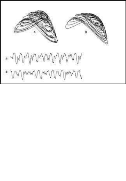
The Glass model (graph A) and the logistic model (graph B) are compared in

Figure 4.11. The delay parameter is m = 40 and a = 0.9 for both models, and b is

set to 0.18 for the Glass model and 0.4 for the logistic model. The similarities are

striking, both in the two-dimensional attractors as well as in the chaotic oscillations,

presented in the lower part of the ﬁgure.

FIGURE 4.11: Comparing the Glass (A) and the logistic (B) delay models

(m = 40)

Various general models were also tested, with similar results. Such general models

are of the form

t+1

= ax

+ F(x

t−m

)

Examples of speciﬁc models that exhibited behaviour similar to that of the Glass

and the delay logistic models in the chaotic region are:

LG2 x

t+1

= ax

+ bx

t−m

(1 − x

t−m

)

LG3 x

t+1

= ax

+ bx

t−m

(1 − x

t−m

)

GRM1 x

t+1

= ax

+ b

t−m

(1 − x

t−m

)

1 − (1 − c)x

t−m

Gauss x

t+1

= ax

+ be

−c(x

t−m

−k)

Gompertz x

t+1

= ax

− bx

t−m

ln(x

t−m

)

(4.15)

We refer to the ﬁve models as delay LG2, delay LG3, delay GRM1, delay Gauss

and delay Gompertz respectively. Chaotic behaviour is expressed for the following

values of the parameters:

In all these cases, the attractors have the same shape as that illustrated in Fig-

ure 4.11.

A diﬀerent chaotic behaviour is exhibited by the following delay exponential

model:

t+1

= x

+ bx

t−m

−cx

t−m

(4.16)

The Delay Logistic Model 91

TABLE 4.2: Parameter values on which various

delay models exhibit chaotic behaviour

Model LG2 LG3 GRM1 Gauss Gompertz

a 0.9 0.9 0.95 0.9 0.9

b (c, k) 0.3 0.243 0.1 (0.84) 0.17 (4, 0.7) 0.28

Model (4.16) gives a relatively stable limit cycle for various values of the parameters.

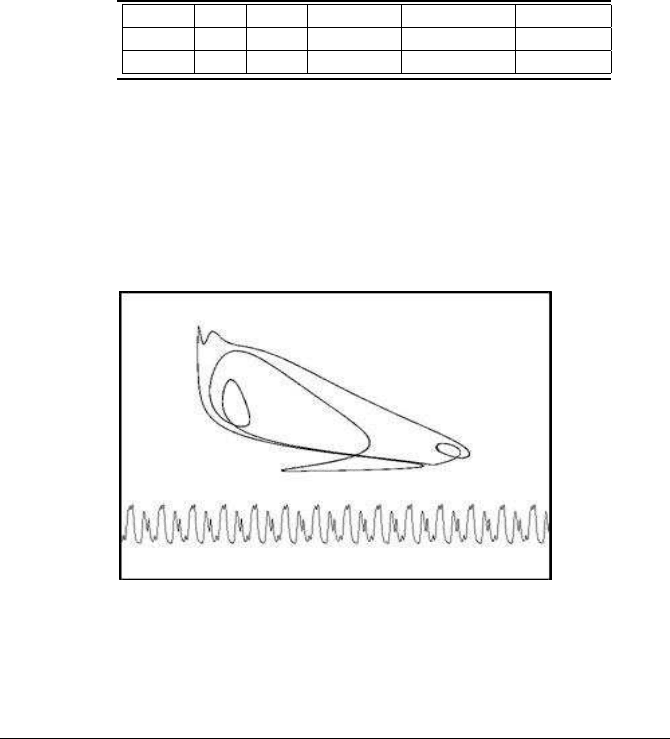
Figure 4.12 illustrates this limit cycle and the related oscillations when the para-

meters of the model take the values a = 0.9, b = 3.2 and c = 0.8. A shape like that

of a pigeon drawn by a modern painter appears.

FIGURE 4.12: The delay exponential model

4.8 Another Delay Logistic Model

A somewhat diﬀerent delay logistic model is given by the following diﬀerence

equation:

t+1

= bx

t−m

+ ax

(1 − x

) (4.17)

When m = 1, this system reduces to a system equivalent to that of the H´enon

model:

t+1

= bx

t−1

+ ax

(1 − x

) (4.18)

The analysis of system (4.18) when b = −1 shows that it has a stable ﬁxed point

92 Chaotic Modelling and Simulation

when

x = 1 −

which turns into the period-2 orbit with:

x =

a + 2 ±

√

(a − 6)(a + 2)

The H

enon model is usually presented in another form, as a two-dimensional

model expressed by a system of diﬀerence equations:

t+1

= by

+ 1 − ax

t+1

= x

(4.19)

However, note that the second equation of (4.19) implies that y

= x

t−1

. We can

therefore substitute this into the ﬁrst equation, and then the following delay equation

results:

t+1

= bx

t−1

+ 1 − ax

(4.20)

Equation (4.20) is equivalent to (4.18), as can be easily observed in Figure 4.13(b).

The small attractor produces the large attractor by rescaling and translation. The

large attractor is the (x

, x

t+1

) image produced by equation (4.20) when a = 1.4 and

b = 0.3. The small attractor is the one produced by equation (4.18) when a = 3.17

and b = 0.3.

(a) Delay cosine-H

enon (b) Delay logistic-H

enon

FIGURE 4.13: Delay logistic and delay cosine H

enon variants

In Figure 4.13(a), the two attractors look as if they were produced by reﬂection

and translation of one to the other. The attractor on the top right of Figure 4.13(a)

is the H

enon attractor provided by the system (4.19). The cross near this attractor is

The Delay Logistic Model 93

located at the origin (0, 0), whereas the cross close to the attractor on the left of the

same ﬁgure is located at (−π, −π). This attractor results from the system

t+1

= by

+ a cos(x

)

t+1

= x

(4.21)

and its corresponding delay equation

t+1

= bx

t−1

+ a cos(x

) (4.22)

This system looks very diﬀerent from (4.19), algebraically, yet the attractors are very

similar. The attractor in Figure 4.13(a) is formed when b = 0.3 and a = 3.22.

Equation (4.22) retains some of the properties of the H

enon map, but it also con-

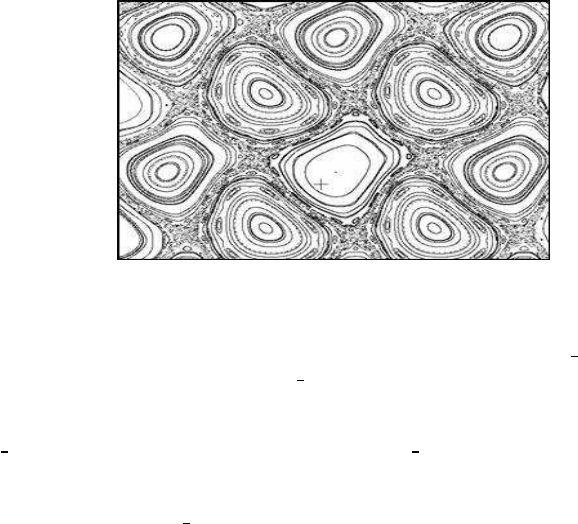
tains other interesting properties, presented in Figure 4.14 (a = −0.4, b = −1). The

map (4.21) is an area-preserving map, as its Jacobian is J = b = −1. The inﬂuence

of the cosine function in the delay equation is clear: The various forms are repeated

many times by following 45

◦

and 135

◦

degrees of symmetry.

FIGURE 4.14: Chaotic patterns of the delay cosine model

Figure 4.15(a) shows the bifurcation diagram (a, x) for 0 < a <

+ 0.1 and

b = −1. The parameter value a =

gives rise to an interesting carpet-like form

(Figure 4.15(b)). An inﬁnite number of islands are included inside the chaotic sea.

Another carpet-like attractor appears in Figure 4.16(a). Here b = −1 and a =

− 0.5. As a is less than the characteristic value

, the islands cover more space

inside the chaotic sea. The chaotic sea almost disappears in Figure 4.16(b). The

islands have now become very ordered geometric structures, and cover almost the

entire plane. Here a =

− 1.5.

There is a systematic way of drawing these graphs. The center of the square-like

forms is located at distances proportional to π, whereas the outer dimension of these

squares is also equal to π. The squares are also related to each other in terms of their

creation over time. With the exception of the central square, all the other squares are

generated in groups of four.