Seuront L. Fractals and Multifractals in Ecology and Aquatic Science

Подождите немного. Документ загружается.

44 Fractals and Multifractals in Ecology and Aquatic Science

Box 3.3 MovEMEnt PAttERnS AS CoRRELAtED RAnDoM WALkS

The correlated random walk (CRW) model has proved its worth in many applications

(Kareiva and Shigesada 1983; Cain 1990, 1994; Turchin 1991). Here, the applicability of CRW

to describe organism movement behavior is illustrated using the movement patterns of the

ocean sunsh, Mola mola, investigated in Section 3.2.1.2. CRW formulation assumes that

move lengths and turning angles are not correlated serially. This was tested by calculating

the autocorrelation function (ACF) and the Ljung–Box Q-statistic for all lags up to six moves

for move length (Turchin 1998). Angular correlation was determined by dening sequential

turns as left or right and performing a run test to check for nonrandomness (Turchin 1998).

For each individual Mola mola, move lengths and turning angles were pooled together within

two groups corresponding to the trajectories recorded during daylight hours and during the

night to calculate an average expected net squared displacement and 95% condence intervals

using a bootstrap simulation of 1000 iterations. Net squared displacements were used because

of the prohibitive difculty inherent in calculations necessary to predict nonsquared displace-

ment (McCulloch and Cain 1989) and because they show a linear relationship with time and

thus are directly related to the rate of population spread (Turchin 1998).

180,000

150,000

120,000

90,000

60,000

30,000

050

Number of Moves

Net Squared Displacement

100 150 200 250

180,000

150,000

120,000

90,000

60,000

30,000

050

Number of Moves

100 150 200 250

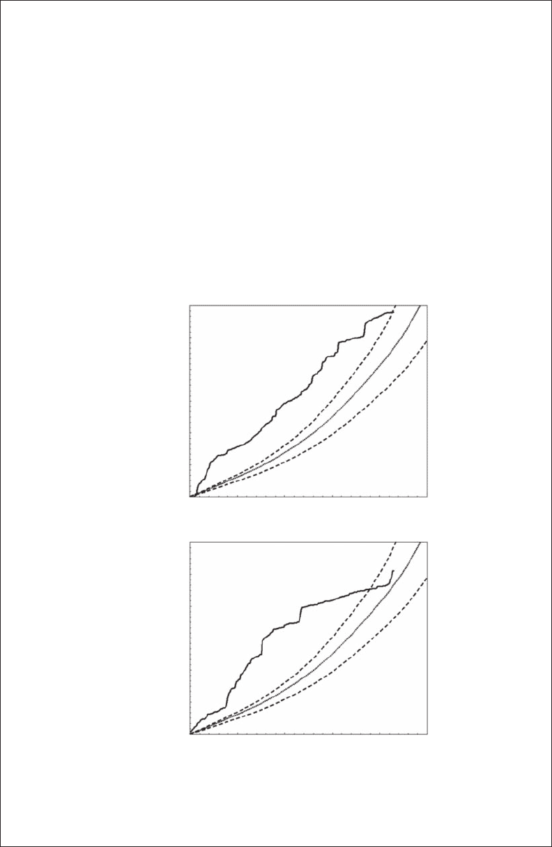
Figure 3.b3.1 Examples of observed (continuous thick line) and expected (dotted line) net squared

displacements in case of a correlated random walk (CRW) model for diurnal (A) and nocturnal

(B) movements of individual eight (see Figure 3.6). The dashed lines are the upper and lower limits of

the 95% condence interval.

2782.indb 44 9/11/09 12:03:58 PM

Self-Similar Fractals 45

We calculated the expected net squared displacement

following Kareiva and Shigesada

(1983):

Rnll

222

−













(3.B3.1)

where

(km

) is the squared displacement from the rst location, n the number of moves

from the rst location, l the mean move length (km), and c the mean of the cosines of the turn-

ing angles. The total number of moves per path simulated by the model varied among Mola

mola tracks and was equal to the largest number of moves taken by an M. mola in a given

track. The observed net squared displacements were then compared to the value predicted by

the CRW model (Figure 3.B3.1).

It is usually unambiguous if the M. mola t the model or not (Figure 3.B3.1A), but in some

cases the track crossed the 95% condence interval for some portion of the displacement

(Figure 3.B3.1B). To determine if M. mola t the model, we used the I statistics as an objective

index of the proportion of observations that lie outside of the 95% condence intervals of the

model prediction (Austin et al. 2004):

Ei Oi

Ei Ei

Ei Oi

=×

−

(

)

−

+×

−

(

() ()

))

−













∑

Ei Ei

() ()

(3.B3.2)

where

in=1, ,

are the successive moves;

j =1

Oi Ei

() ()>

and

j =0

Oi Ei

() ()<

;

k =1

Oi Ei

() ()>

and

k =0

Oi Ei

() ()<

;

and

are the upper and lower limits of the 95%

condence intervals;

Oi()

the observed

, and

()

, and

()

the expected lower,

upper, and mean

values. The 95th percentile of the expected

is used as the critical

value and compared to the observed trajectories. Paths with an l value greater than the criti-

cal value were considered to signicantly differ from the CRW model. The movements of

the eight M. mola were systematically underpredicted by the CRW model (Figure 3.B3.1) for

daytime and nighttime movements. Sunsh then exhibited greater directionality of movement

and longer move lengths than expected under the CRW assumption.

Benhamou (2004) also stated that “animals’ random search paths, at least when they are mod-

eled as correlated random walks, are not fractal.” Although this is common sense since correlated

random walks are classical (nonfractal) models, they may erroneously return a fractal signature

(that is, a linear behavior of the log-log plot of L(d ) vs. d), especially when the range of scales avail-

able in the analysis (that is, the number of data points) is limited (Turchin 1996; Benhamou 2004),

which is a recurring issue in ecological studies and may lead to what is called apparent fractality

(Hamburger et al. 1996; Halley et al. 2004). A typical example of a mishandling of both correlated

random walks and fractal analysis is provided by, for example, Uttieri et al. (2005). Despite the non-

fractal character of correlated random walks (Turchin 1996; Benhamou 2004); Uttieri et al. (2005)

analyzed the fractal properties of simulated three-dimensional correlated random walks of increas-

ing length (5,000, 10,000, and 50,000 points) using a three-dimensional box-counting method (see

Section 3.2.2). Although they did not provide any gure to support their ndings, they claim that

“the regression lines of the log-log plots t the points with good accuracy” (i.e. r

≈ 0.99) and their

fractal analysis returned decreasing fractal dimensions (1.69, 1.48, and 1.41), interpreted as the

expression of “a decrease in morphological complexity of the trajectories.” These results are irrel-

evant given the nonfractal nature of correlated random walks. They may nevertheless be explained

by the shape of the log-log plots of L(d ) vs. d returned by the fractal analysis of a correlated random

2782.indb 45 9/11/09 12:04:11 PM

46 Fractals and Multifractals in Ecology and Aquatic Science

walk (Figure 3.8A). These plots can indeed appear relatively, even very, linear depending on the

parameters used to simulate the correlated random walk (Figure 3.8A). As a consequence, in some

instances, linear ts can return very high values of r

and hence lead to identication as linear a

nonlinear plot of log L(d ) vs. log d (Figure 3.8B). It is also likely from their subsequent analysis of

the three-dimensional swimming path of the water ea Daphnia pulex that Uttieri et al. (2005) did

not use any objective criteria to choose the range of scales used to estimate fractal dimensions (see

their Figure 4C).

To avoid erroneously considering a correlated random walk as returning a fractal signature

prior to fractal analysis, it is then necessary to test, as a null hypothesis, whether a correlated ran-

dom walk model adequately describes the path properties (Box 3.3). If the null hypothesis is to be

rejected, it is still necessary to assess objectively the nature of the signature of the log-log plot of

L(d ) vs. d (see Box 3.2 and Chapter 6). This is critical to ensure the relevance of fractal analysis, as

a number of previous works on fractal analysis have implicitly made the assumption that the slopes

of log-log plots were linear without preliminary critical assessment (for example, Crist et al. 1992;

Crist and Wiens 1994; With 1994; Laidre et al. 2004; Uttieri et al. 2005, 2007). It is stressed that the

“fractal signature” of correlated random walks can only be erroneously considered as the expres-

sion of a fractal behavior if the scaling range is narrow, that is, typically smaller than one decade

(see Figure 3.8A).

3.2.2 bo x di m E n s i o n , D

3.2.2.1 theory

This procedure, like the divider method, can be used to measure the fractal dimension of a curve

(Longley and Batty 1989). In addition, it can be applied to overlapping curves (Peitgen et al. 1992)

and structures lacking strict self-similar properties such as vegetation (Morse et al. 1985). Formally,

the method nds the “d cover” of the object—that is, the number of boxes of length d (or circles of

radius d) required to cover the object (Voss 1988). A more practical alternative is to superimpose

a regular grid of pixels of length d on the object and count the number of “occupied” pixels. This

procedure is repeated using different values of d. The volume occupied by a curve is then estimated

with a series of counting boxes spanning a range of volumes down to some small fraction of the

entire volume. The number of occupied boxes increases with decreasing box size, leading to the

following power-law relationship (Loehle 1990):

N(d ) = kd

−D

(3.13)

where d is the box size, N(d ) is the number of boxes occupied by the curve, k is a constant, and

is the box fractal dimension. D

is estimated from the slope of the linear trend of the log-log

plot of N(d ) versus d. Note that Equation (3.13) can indifferently be used with one-, two- or three-

dimensional objects.

It is stressed that both interior and border boxes contribute to the total number of boxes N(d )

intersected by the set. Interior boxes are fully contained within the fractal set; that is, they only

contain a part of the set. In contrast, border boxes contain at least one white pixel and contain or

adjoin at least one black pixel. Thus,

N(d ) = N

(d ) + N

(d ) (3.14)

The border-box fractal dimension, D

, is then estimated as the linear trend of the log-log plot of

(d ) versus d. The interior-box fractal dimension, D

, is similarly estimated as the linear trend of

a log-log plot of (N(d ) − 0.5N

(d )) against d . The substraction term is necessary to avoid an overes-

timate of the area of the structure at large box sizes since the border boxes are not entirely lled by

2782.indb 46 9/11/09 12:04:13 PM

Self-Similar Fractals 47

the set (Kaye 1989). Note that the border box dimension D

is strictly equivalent to the boundary

fractal dimension D

(see Equation 3.12, Section 3.2.1.1).

In the case of real data sets, one must always work with a nite set

(which may or may not be

interpreted as a sample of the points from some innite set). The above limit of a nite set is thus

always zero (D

= 0) because eventually d will be so small that there will only be one point in each

occupied cell. Once d becomes sufciently small, N(d ) becomes equal to the number of points in

the set, and the limit above this is (see Equation 3.9):

→

lim

log()

log( /)

(3.15)

where D

= 0, because

log()N

is a constant and

log( /)1

→+∝

→0

. This is a consequence of

all nite sets being zero-dimensional; they have the same dimension as a single point (see Section

2.2.1 for further details). In practice, the dimension D

will thus be estimated using a range of d

values that are always greater than the resolution of the studied set, which can be signicantly

greater than a pixel in the case of digitized objects. This potential limitation has to be taken into

account when writing (or, more prosaically, using) a computer program for automatic estimation of

. In addition, this method does not take into account the frequency with which the set in question

might visit the covering cells, and thus local properties of the set (that is, properties pertaining to

neighborhoods of individual points) are not distinguishable. It will nevertheless be shown below

with the introduction of the cluster dimension, D

, and the family of dimensions related to frequency

distributions that this difculty can easily be overcome.

Finally, for Euclidean objects, Equation (3.13) directly denes their dimensions. A number of

boxes proportional to d

−1

are needed to cover a smooth line, and proportional to d

−2

and to d

−3

cover a curve convoluted on a plane and in a volume, respectively.

3.2.2.2 case study: burrow morphology of the grapsid crab, Helograpsus Haswellianus

3.2.2.2.1 Study Organism

The Australian grapsid crab or mud shore crab, Helograpsus haswellianus (Figure 3.9A) is common

in sheltered bays and estuaries along the eastern coastline of Australia from Queensland south to

Tasmania. H. haswellianus is a nocturnal species often found well above high-tide level in areas of

mud, and forages widely on the shore between tides (Breitfuss 1982). These crabs can be especially

abundant on salt-marsh ats (Figure 3.9B), and some are found well upriver in fairly low salinity

areas (Marsh 1982). They are also found among mangrove roots, especially those of Avicenna

marina, often in association with the red-ngered marsh crab, Sesarma erythrodactyla, and the

semaphore crab, Heloecius cordiformis (Campbell and Griffen 1966).

H. haswellianus burrow in a variety of soft sediments, ranging from dirty sand to moist clay, and

shelter under debris or rocks. Such burrowing may create quite distinct systems of interconnecting

burrows in muddy estuaries. Burrows increase the surface area available for tidal inltration of sea-

water (Smith et al. 1991), thus maintaining a critical chemical pathway between anoxic sediments

and seawater (Nomann and Pennings 1998), and provide crabs daytime protection from desiccation

and predation as well as being used for courting, breeding, and molting (Morrisey et al. 1999).

Typically, studies of burrow shape have examined metrics such as burrow system shape, burrow

system area, number of segments, linearity, turn angle, number of branches, segment length, and

branch length; see Romaña et al. (2005) for a detailed explanation of these terms. However, because

the interactions between these variables are not clear (Le Comber et al. 2006), recent studies have

begun to use fractal dimension to provide a single measure of shape that has the desirable advan-

tage of being independent of burrow length (Puche and Su 2001; Sumbera et al. 2003; Romaña and

Le Comber 2004).

2782.indb 47 9/11/09 12:04:16 PM

48 Fractals and Multifractals in Ecology and Aquatic Science

3.2.2.2.2 Experimental Procedures and Data Analysis

The morphology of H. haswellianus burrows was investigated by pouring a liquid epoxy resin

into openings, leaving it to harden, and digging the cast out after 36 hours. The three-dimensional

complexity of the burrows (Figure 3.9C,D,E,F) was investigated using Equation (3.13), a proce-

dure previously successfully applied to other branched structure–like vegetation (Morse et al.

1985; Critten 1993; Zeide and Gresham 1991; Zeide 1998; Eshel 1998; Alados et al. 1998, 1999;

Forountan-pour et al. 1999, 2000, 2001). Seaweeds (Corbit and Garbary 1995; Kübler and Dugeon

1996; Davenport et al. 1996), corals (Basillais 1997), sponges (Kaandorp 1991; Kaandorp and

de Kluijver 1992; Abraham 2001) and gorgonians (Burlando et al. 1991; Mistri and Ceccherelli

1993) provide instances of marine organisms that have been shown to have fractal properties

using the box-counting method (Figure 3.10A,B,C). However, because the fractal characterization

of three-dimensional (3D) structures would have nontrivially requested a rebuild of the digitized

version of the original burrow, the problem has been simplied by obtaining two orthogonal

photographic images of the burrow and subsequently estimating their two-dimensional (2D)

fractal dimensions.

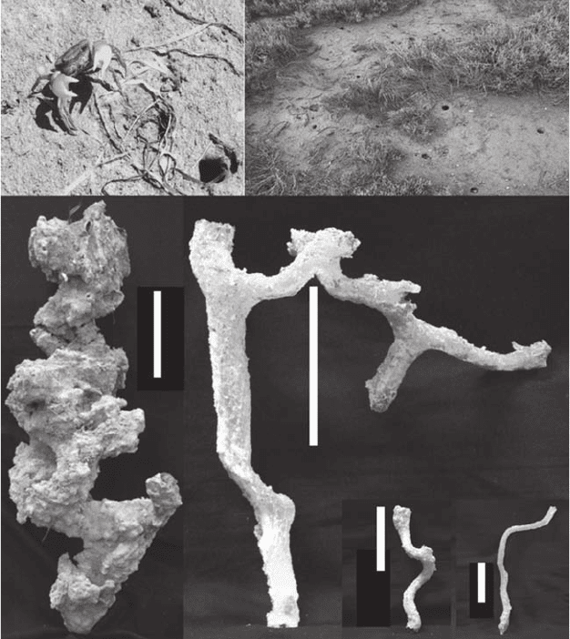
Figure 3.9 (A) Grapsid crab, Helograpsus haswellianus, shown together with (B) its typical salt-marsh

environments, and illustrations of the resin casts sampled at (C) Goolwa, (D) Torrens Island, (E) Middle

Beach, and (F) Port Noarlunga. The scale bars represent 10 cm. (Courtesy of G. Katrak, Flinders University,

Australia.)

2782.indb 48 9/11/09 12:04:19 PM

Self-Similar Fractals 49

H. haswellianus burrow morphology was investigated from four distinct South Australian salt

marshes located at Goolwa (Figure 3.11A; N = 2), Torrens Island (Figure 3.11B; N = 7), Middle Beach

(Figure 3.11C; N = 13), and Port Noarlunga (Figure 3.11D; N = 14). The vegetation of the four sites is dom-

inated by Sarcocornia quinqueora and characterized by the presence of Halosarcia haswellianus.

3.2.2.2.3 Results

All the burrows investigated exhibited very strong scaling behavior for Equation (3.13) (Figure 3.10D)

with the coefcient of determination r

ranging from 0.96 to 0.99 over the whole range of available

scales, that is, between 0.5 and 15 cm, and 0.5 and 50 cm for the smallest and largest burrows, respec-

tively. This is illustrated by the log-log plot of N(d ) versus d (Figure 3.10D) estimated for the burrows

shown in Figure 3.10A,B,C. The two-dimensional fractal dimensions D

(0°) and D

(90°) were never

signicantly different (covariance analysis, p > 0.05; Zar 1996) for the burrows investigated at Goolwa

and Port Noarlunga, and only one burrow each at Torrens Island and Middle Beach exhibited sig-

nicant differences between D

(0°) and D

(90°) (Figure 3.12). The resulting mean two-dimensional

fractal dimensions ranged between 1.59 and 1.62 at Goolwa (

=± ±1.60 0.02; SDx

), 1.34 and

1.67 at Middle Beach (D

= 1.56 ± 0.05), 1.39 and 1.54 at Port Noarlunga (D

= 1.49 ± 0.03), and

1.50 and 1.62 at Torrens Island (D

= 1.55 ± 0.04). Signicant differences were found between the

fractal dimensions obtained from the burrow resin casts sampled at Goolwa, Middle Beach, Port

Noarlunga, and Torrens Island (Kruskal-Wallis test, p < 0.01). A subsequent multiple-comparison

procedure showed that the fractal dimensions estimated at Middle Beach and Torrens Island were

–0.5 0.0

Log δ

0.5 1.0 1.5

Log N (δ)

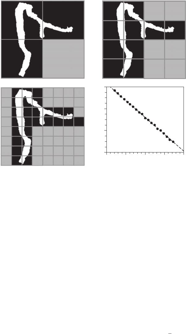
Figure 3.10 Schematic illustration of the box-counting method used to describe the complexity of burrow archi-

tecture with fractal dimension. Three steps are shown, using three different characteristic scales d

(A), d

(B), and

= 2d

= 4d

. The gray areas are the squares of size that do not include a part of the burrow.

The scaling behavior of the log-log plot of N(d) vs. d for the burrow shown in (A, B, C) is shown in (D).

2782.indb 49 9/11/09 12:04:22 PM

50 Fractals and Multifractals in Ecology and Aquatic Science

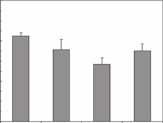
not signicantly different (p > 0.05), but signicantly lower and higher (p < 0.05) than those esti-

mated at Goolwa and Port Noarlunga, respectively. This leads to the identication of three groups

of burrow morphology based on the box dimension D

(Figure 3.13): a group of highly complex

burrows at Goolwa (D

= 1.62 ± 0.02), a group of burrows of intermediate complexity at Middle

Beach and Torrens Island (D

= 1.56 ± 0.05), and a group of less complex burrows at Port Noarlunga

= 1.49 ± 0.03).

3.2.2.2.4 Ecological Interpretation

No signicant differences were found between the fractal dimensions of the burrows investigated

at Port Noarlunga whether the dominant vegetation was Sarcocornia quinqueora (20 to 30%)

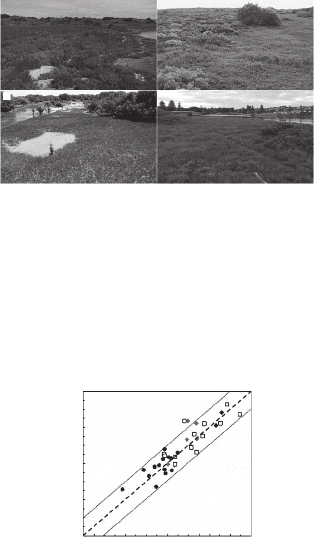
Figure 3.11 Salt-marsh environments where H. haswellianus burrow morphology was investigated in

(A) Goolwa, (B) Torrens Island, (C) Middle Beach, and (D) Port Noarlunga. (Courtesy of G. Katrak, Flinders

University, Australia.) (See color insert following page 80.)

1.7

1.6

1.5

(90°)

(0°)

1.4

1.3

Figure 3.12 Comparisons of the two-dimensional fractal dimensions estimated from two orthogonal

projections of the original burrow resin casts sampled at Goolwa (black diamonds), Middle Beach (open

squares), Port Noarlunga (black dots), and Torrens Island (gray diamonds). The dashed line is the rst bisectrix

(0°) = D

(90°), and the dotted lines indicate the corresponding 5% condence intervals.

2782.indb 50 9/11/09 12:04:25 PM

Self-Similar Fractals 51

or Suaeda australis (20 to 35%). This suggests that the qualitative nature of the vegetation cover

does not inuence the complexity of burrows. In turn, the quantitative nature of the vegetation

cover might inuence the complexity of H. haswellianus burrows. The fractal dimensions of the

burrows investigated at Goolwa, Middle Beach, Torrens Island, and Port Noarlunga on substrates

respectively covered at 100%, 85 to 90%, 85%, and 20 to 30% are signicantly decreasing with the

vegetation cover (Figure 3.13). Finally, the nonsignicant differences found between the burrows

investigated at Middle Beach on bare substrate and on a substrate covered by S. quinqueora might

also suggest that within a given site, the percentage of vegetation cover has a rather limited effect

on burrow morphology. The nonsignicant differences found between the two 2D fractal dimension

estimates D

(0°) and D

(90°) (Figure 3.12) indicate that the morphology of H. haswellianus bur-

rows is mainly isotropic, suggesting a fully three-dimensional burrowing behavior.

As burrowing might be thought as a way of foraging underground, the use of fractals to

quantify burrow architecture is conceptually equivalent to the use of fractals to characterize

the complexity of three-dimensional trajectories of swimming organisms (Seuront et al. 2004a,

2004b; Uttieri et al. 2005). As most behavioral metrics are also scale dependent (see Seuront et al.

2004a, 2004b for a review), there is no single scale at which swimming paths can be unambigu-

ously described. As a consequence, when using standard metrics, there is no single scale at which

swimming paths (and burrow morphology) can be compared without leading to potentially spuri-

ous conclusions. Fractal dimension is a natural choice for a measure of burrow shape complexity,

as it is essentially a measure of the extent to which a one-dimensional structure lls a plane, with

low fractal dimension (D

≈

1) describing a burrow that explores relatively little of the surround-

ing area, and high fractal dimension (D

≈

2) describing a burrow that explores the surrounding

area more thoroughly. Fractal dimension seems thus particularly well suited as a measure of

burrow shape when burrows are used for foraging.

3.2.2.3 methodological considerations

The procedure described above can be used to estimate the box dimension of two- and three-

dimensional objects through the superposition of squares (or circles) and boxes (or spheres) of dif-

ferent side lengths and radii to the object of interest. Two potential limitations intrinsically related

to the method have nevertheless been identied in both cases: (1) slight reorientation of the overly-

ing grid can produce different values of N(d ) (Equation 3.13; Appleby 1996), and (2) the values of

box dimensions may be positively correlated to the object length (Erlandson and Kostylev 1995).

1.8

1.6

1.4

Fractal Dimension D

1.2

GMB

Sampling Site

PN TI

Figure 3.13 Fractal dimensions of burrows architecture, estimated as D

= [D

(0°) + D

(90°)]/2 at Goolwa

(G), Middle Beach (MB), Port Noarlunga (PN), and Torrens Island (TI). D

(0°) and D

(90°) are the fractal

dimensions of two random, orthogonal views of the burrows resin casts.

2782.indb 51 9/11/09 12:04:27 PM

52 Fractals and Multifractals in Ecology and Aquatic Science

Consequently, the behavior of Equation (3.13) will be biased, as will be the subsequent box dimen-

sion estimates.

As described for the divider dimension, a distribution of the box dimension, D

, can be obtained

from random replicates of the grid placements in the box-counting algorithm. For two-dimensional

objects (see, for example, Figure 3.10), the initial 2D orthogonal grid is rotated in 5° increments

from a = 0° to a = 45°. Alternatively, for three-dimensional objects, the initial 3D orthogonal grid

is rotated in 5° increments from a = 0° to a = 45° in the x − y plane and from b = 0° to b = 45°

in the x − z plane. The resulting distributions of dimensions can thus be used as estimates of the

box dimensions of the two- and three-dimensional objects. The limitation of the method raised by

Erlandson and Kostylev (1995)—that is, values of box dimensions might be positively correlated to

a path’s length—can be addressed by comparing the box dimensions of randomly chosen subsets of

decreasing length within the same set.

Applying these procedures to nine swimming trajectories of the water ea, Daphnia pulex, rang-

ing in duration from 1.5 to 4 minutes; Seuront et al. (2004a) did not nd any effects related to

the orientation of the three-dimensional grid or to the length of the trajectories. It is nevertheless

advised that this potential bias should be thoroughly investigated to ensure the robustness of any

box dimension estimated through Equation (3.13).

3.2.2.4 theoretical considerations

3.2.2.4.1 Two-Dimensional versus Three-Dimensional Fractal Dimensions

The ability to characterize 3D paths based on 2D projections of these paths is an attractive proposition,

as the reduction in complexity of both the data-gathering equipment and the analysis procedures

is signicant. However, the reliability of conclusions based on such a procedure is not clear. The

consequences of extrapolating fractal dimensions estimated in a 2D framework to three dimensions

have been assessed by the following:

Testing the validity of the extrapolation procedures proposed in the literature (Morse et al. •

1985; Shorrocks et al. 1991; Gunnarsson 1992).

Investigating the potential disparity among the fractal dimensions estimated from the three •

orthogonal two-dimensional projections of three-dimensional objects.

Demonstrating the necessity of three-dimensional isotropy of a given object as a prerequi-•

site for extrapolating two-dimensional fractal information into a three-dimensional space.

The philosophy behind the extrapolation of two-dimensional fractal estimates to three dimen-

sions is simple. Morse et al. (1985) described a box-counting method for estimating the fractal

dimension of vegetation habitats (2 ≤ D

≤ 3, where the subscript 3 indicates a fractal object embed-

ded in a three-dimensional space). Consider now the problem of estimating the fractal dimension

of a tree. In theory, a three-dimensional grid system could be superimposed on the tree and the

size of “counting-cubes” varied. Such a procedure would nevertheless require a digital reconstruction

of the tree from photographs, which is still extremely challenging (see, for example, Shlyakhter et al.

2001). Morse et al. (1985) simplied the problem by obtaining a 2D photographic image of the

habitat, the fractal dimension of which was determined using the box-counting method (1 ≤ D

≤ 2,

where the subscript 2 indicates a fractal object embedded in a two-dimensional space). Following

Mandelbrot (1983), they determined heuristic lower (D

3min

= D

+ 1) and upper (D

3max

= 2D

) limits

of the “habitat” fractal dimension under the assumption that the photograph is a randomly placed

orthogonal plane. This procedure has subsequently been used to estimate the fractal dimensions of

various habitats (for example, Shorrocks et al. 1991; Gunnarsson 1992). However, it is argued here,

on the basis of both simple theoretical and empirical arguments, that the use of this procedure to

characterize three-dimensional movement pathways is highly questionable. This issue is illustrated

using records of the mud shore crab burrow morphology (Section 3.2.2.2) and the three-

dimensional motion behavior of the water ea, Daphnia pulex (Box 3.4, Figure 3.14).

2782.indb 52 9/11/09 12:04:28 PM

Self-Similar Fractals 53

Box 3.4 thREE-DIMEnSIonAL AnALySIS oF thE

WAtER FLEA,

DAPhnIA PuLEx

, SWIMMInG PAth

A clone of Daphnia pulex was cultured in aged tap water under cool white uorescent bulbs,

in a 16–8 light–dark cycle. The cultures were maintained at the experimental temperature

(20°C) and fed every day with a 1:1 mixture of the green algae Ankistrodesmus sp. and

Scenedesmus sp. at a nal concentration of about 5 × 10

cells/ml

−1

. Algae were grown in mul-

tiple 250 ml batch cultures under cool white uorescent bulbs, in an 18–6 light–dark cycle, at

20°C, in Bold’s basal medium.

All paths analyzed here are the movements of solitary D. pulex swimming in the 5-liter

(18 × 18 × 15.5 cm high) Plexiglas recording vessel of the CritterSpy, a high-resolution 3D

recording system. All recordings were made with animals swimming in an algal concentra-

tion of 5 × 10

cells/ml

−1

, which is an intermediate food concentration, well below D. pulex’s

incipient limiting concentration (Lampert 1987). The test chamber was illuminated with a

diffused, ber-optic light placed 0.5 meter directly overhead that resulted in an illumination

of about 12 µEm

−2

−1

in the vessel, approximately equal to full daylight. At least 1 hour prior

to experiments, adult, gravid females (

21 02..±

mm) were transferred from their culturing

vessels and acclimated to experimental light and food conditions in holding vessels. A single

animal was then transferred from its holding vessel to the recording chamber with a large-

bore pipette and allowed to acclimate for at least 10 minutes before recording began.

The CritterSpy uses a schlieren optical system consisting of a collimated red laser beam

(λ = 623 nm) that serves as the light source for two orthogonally mounted video cameras, two

frame-number generators, two 20” video monitors, and two VHS videocassette recorders;

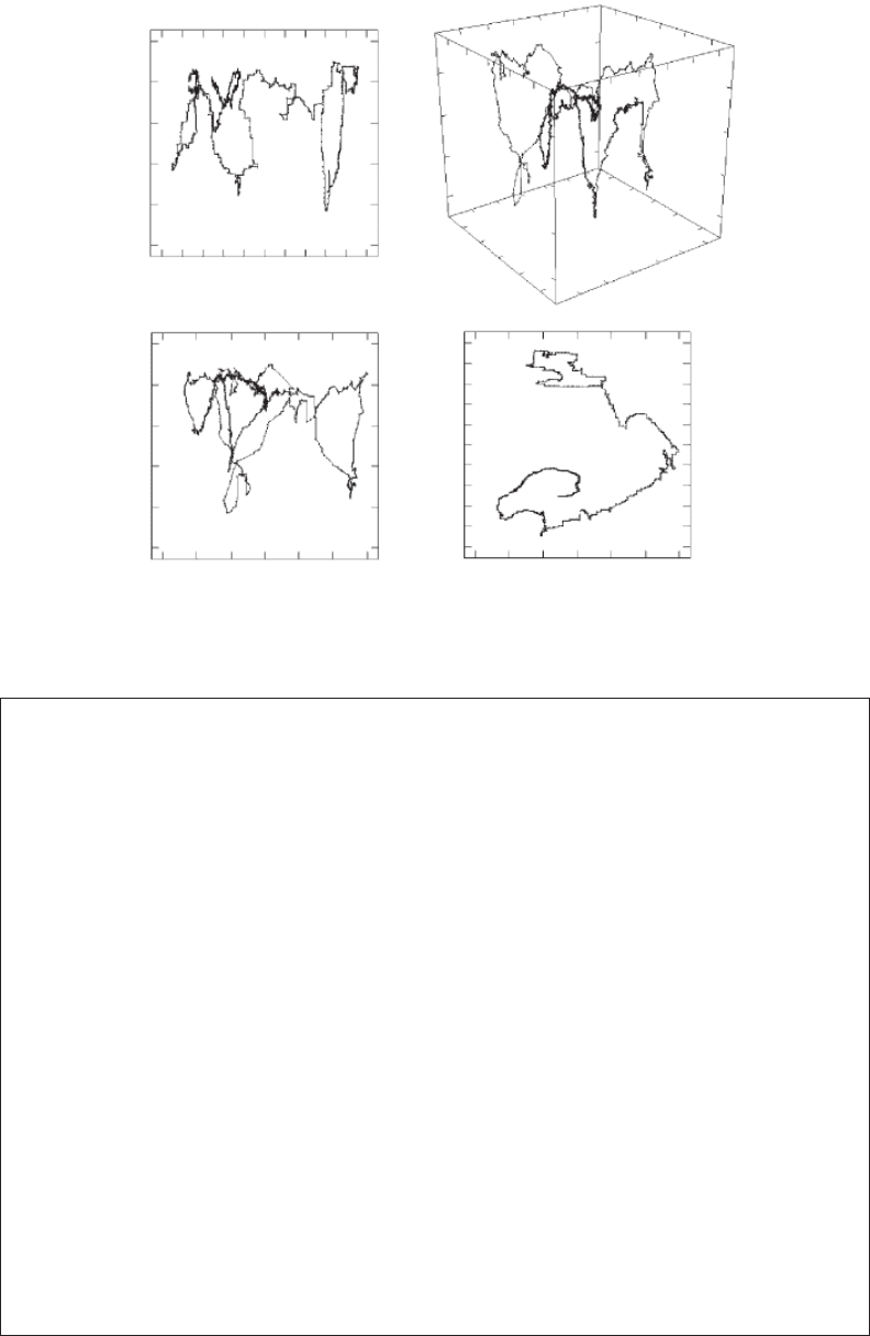
Figure 3.14 Illustration of the three-dimensional swimming path of the water ea, Daphnia pulex (A), and

the corresponding two-dimensional projections on the planes x − y (B), x − z (C), and y − z (D).

2782.indb 53 9/11/09 12:04:31 PM