Seuront L. Fractals and Multifractals in Ecology and Aquatic Science
Подождите немного. Документ загружается.

24 Fractals and Multifractals in Ecology and Aquatic Science
where the sampling fractal dimension D
FS
veries D
FS
> 0 for D
S
> c
F
− D
T
. The extreme case D
FS
= 0
corresponds to single points isolated in the sample; when D
S
> c
F
and D
S
> c
F
, S is present and absent
in the sample, respectively.
The so-called fractal dimension and codimension referred to in the previous section are com-
monly estimated from the regression slope of a log-log power-law plot; see, for example, Equations
(2.1), (2.3), (2.10), (2.14), and (2.15). However, this procedure is not necessarily as straightforward
as it may appear at rst glance and relies on many successful consecutive steps, the minimum
prerequisite being to choose the appropriate analysis techniques (that is, an appropriate power
law). To achieve this goal, one needs rst to know the difference between self-similar and self-
afne fractals as well as to identify the limits of fractal analysis, such as those related to both
anisotropy and nonstationarity conditions often encountered in aquatic ecology. Objective crite-
ria are also needed to select the appropriate range of scales to include in the regression analysis.
Then comes the question of distinguishing scaling from multiple scaling behaviors. The nal
question that needs to be addressed is to know whether fractal concepts can be powerful enough
to measure the extreme complexity emerging from the highly intermittent patterns encountered
in both terrestrial and aquatic ecosystems.
2782.indb 24 9/11/09 12:03:19 PM
25
3
Self-Similar Fractals
As stated in Chapter 2, fractals are dened to be scale-invariant geometric objects. However, scale
invariance can be dichotomized into self-similar and self-afne fractals. Strictly speaking, an object
is called self-similar if it may be written as a union of rescaled copies of itself with the rescaling iso-
tropic (that is, uniform in all directions). Regular fractals such as the Koch snowake (Figure 2.5a)
and the Sierpinski carpet and gasket (Figure 2.8) display exact self-similarity. Random fractals such
as the random Koch snowake (Figure 3.1) display a weaker, statistical version of self-similarity
or, more generally, statistical self-similarity. More formally, a geometric object is called self-afne
if it may be written as a union of rescaled copies of itself, where the rescaling is anisotropic (that
is, dependent on the direction). Thus the trace of particulate Brownian motion in two-dimensional
space is self-similar, whereas a plot of the x coordinate of the particle as a function of time is self-
afne (Figure 3.2).
3.1 selF-similarity, Power laws, and the Fractal dimension
Mathematical fractals exhibit exact self-similarity across all spatial or temporal scales, such that suc-
cessive magnications reveal an identical structure. A self-similar object is composed of N copies of
itself (with possible translations and rotations), each of which is scaled down by a scale ratio d in all
directions of the D
E
dimensional available space. More formally, consider a set S of points at posi-
tions
xxxx
D
E
=(, ,, )
12
in Euclidean space of dimension D
E
. Under a similarity transform with a
scale ratio d (0 < d < 1), the set S becomes d S with points at positions
δδδδ
xxxx
D
E
= (
12
,,,).
A
bounded set S is self-similar when S is the union of N nonoverlapping subsets, each of which is iden-
tical (under translations and rotations) to d S. A basic example of a self-similar fractal is the Cantor
set (Cantor 1883). Consider a line segment ([0, 1]), divide it into thirds, and remove the central part.
Repeat the procedure on the two remaining thirds, and after an innite number of iterations, one
converges to a set of points or Cantor set, also referred to as Cantor dust (Figure 3.3).
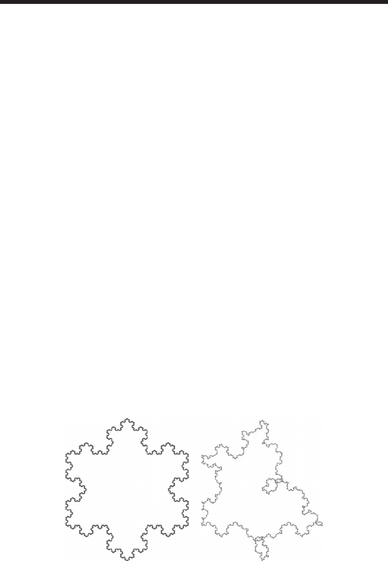
AB
Figure 3.1 Difference between self-similar and statistical self-similar fractals. The Koch snowake
(A) displays exact self-similarity, while the random Koch snowake (B) displays a weaker, statistical version
of self-similarity, referred to as self-afnity.
2782.indb 25 9/11/09 12:03:23 PM
26 Fractals and Multifractals in Ecology and Aquatic Science
The construction rules of such simple sets lead to a simple way to calculate their related fractal
dimensions. In the case of the Cantor set (which can be easily extended to other geometrical frac-
tals), at stage n of the construction process, the set is characterized by 2
n
intervals of length 3
−n
; its
total length is thus (2/3)
n
. At the limit n → ∞, the length of the Cantor set is then nil, and its topo-
logical dimension is D
T
= 0. To estimate its fractal dimension, consider a cover of the sets by line
segments of length d
n
= (1/3)
n
. From the previous statements, it comes that only N(d
n
) = 2
n
segments
cover a part of the Cantor set. The length of the Cantor set can thus be expressed as L
n + 1
= (2/3) L
n
,
whose solution is of the form:
L
nn
D
F
()
δ
=
−
δ
1
(3.1)
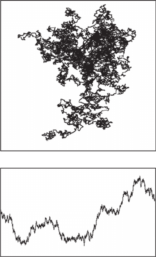
A
X (t)
Time
Bm (t)
Y (t)
B
Figure 3.2 Difference between self-similar and self-afne fractals. The trace of a Brownian motion in a
two-dimensional space is self-similar (A), whereas the plot of the x coordinate of the particle as a function of
time is self-afne (B). The major difference is that the rescaling is dependent on the direction in the latter case;
that is, the horizontal and the vertical axes do not have the same meaning in (B).
2782.indb 26 9/11/09 12:03:25 PM
Self-Similar Fractals 27
The number of length elements required to cover the total length is given by L(d
n
)/d
n
and equal to:
N
nn
D
F
()
δδ
=
−
(3.2)
The fractal dimension D
F
can nally be generally expressed as:
D
F
= log N(d
n
)/log(1/d
n
). (3.3)
or equivalently:
D
F
= log N(d
n
)/logl
n
(3.4)
where the scale-ratio l is dened as:
l = d
n +1
/d
n
(3.5)
where d
n +1
and d
n
are respectively the length elements required to cover a piece of the Cantor set at
steps n + 1 and n of the construction process. For the Cantor set, l = 3, and the fractal dimension
D
F
= log 2/log 3 = 0.631. A generalization for the areas and volumes of fractal surfaces and volumes
can be easily derived from Equation (3.1) as:
S
nn
D
F
()
δδ
=
−2
(3.6)
and
V
nn
D
F
()
δδ
=
−3
(3.7)
It is stressed here that the fractal dimensions D
F
introduced in Equations (3.2), (3.6), and (3.7) can be
referred to as “fractal line dimension,” “fractal surface dimension,” and “fractal volume dimension,”
respectively. The exponents in Equations (3.1), (3.6), and (3.7) also directly refer to the codimension
concept introduced in Section 2.2.2.1, Equation (2.12).
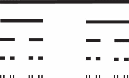
n = 0
n = 1
n = 2
n = 3
n = 4
Figure 3.3 Construction of the Cantor set, by repeated removal of the middle third of each interval; at
each step, there are two elements that are three times smaller, leading to a fractal dimension D
F
= log 2/
log 3 = 0.631.
2782.indb 27 9/11/09 12:03:29 PM
28 Fractals and Multifractals in Ecology and Aquatic Science
A set S is also self-similar if each of the N subsets is scaled down from the whole by a different
similarity ratio d
i
. The fractal dimension D
F
is then given by
δ
i
D
i
N
F
=
∑
=
1
1
(3.8)
which is strictly equivalent to Equation (3.2) when all the d
i
are equal (Voss 1985).
Unlike mathematical fractals, natural objects do not display exact self-similarity.
Nevertheless, many natural objects do display some degree of “statistical” self-similarity, at
least over a limited range of spatial or temporal scales, corresponding to partial self-similarity.
For example, lung branching shows self-similarity over 14 dichotomies, and tree branching
over 8 dichotomies (Schroeder 1991). In addition, the existence of stepwise behavior (that is,
changes in fractal dimension when shifting between scales) implies that in place of true self-
similarity, we observe only partial self-similarity over limited ranges of scales separated by
transition zones, where the environmental properties or constraints acting upon organisms are
probably changing rapidly (Frontier 1987; Seuront and Lagadeuc 1998; Seuront et al. 1999).
This is of prime interest in aquatic ecology since the extent of a given power law (referred to
as the scaling range hereafter) allows the identication of the characteristic scales of organi-
zation of any pattern or process. Several objective procedures devoted to the identication of
scaling ranges (that is, a key step for the result of fractal analysis to be meaningful) will thus
be introduced in Chapter 7.
Statistical self-similarity refers to scale-related repetitions of overall complexity but not of the
exact pattern. Specically, details at a given scale are similar, though not identical, to those seen
at coarser or ner scales. A set S is statistically self-similar if it is composed of N distinct subsets,
each of which is scaled down by a ratio d from the original and is identical in all statistical respects
to dS. The related fractal dimension is still given by Equation (3.1) and Equation (3.2). In that way,
the prevalence of power law with respect to the scale of observation in a certain range is commonly
used to discern a fractal, especially when the scale of similarity is statistical and cannot be identi-
ed by sequential enlargement of segments of the fractal object. A collection of methods devoted to
the characterization of different kinds of self-similar natural objects (for example, branching pro-
cesses such as vascularization, lung systems, or stream orders and discrete patterns such as islands
or pancreatic islets) are provided in Section 3.2.
It should be emphasized that self-similarity is not a prerequisite to applying fractal theory. Self-
similar or statistically self-similar patterns are characterized by fractal dimensions that remain
constant for each subpart of the whole (Mandelbrot 1983; Tricot 1995). Geographic lines, such as
coastlines, are nevertheless very complex curves, whose local dimensions (see Section 2.2.1) are not
the same everywhere. Such curves are not self-similar, not even statistically (Normant and Tricot
1993). As a consequence, we stress that (strictly speaking) fractal does not imply self-similar, and
thus coastlines are not self-similar but fractal. Self-similarity is thus a restrictive point of view.
This has also briey been addressed by Voss (1985), who stressed that “in practice it is impossible
to verify that all moments of the distributions are identical, and claims of statistical self-similarity
are usually based on only a few moments.” This specic point is nevertheless beyond the scope of
this section and will be discussed more extensively hereafter with the introduction of the concept of
multifractals (see Chapter 8).
3.2 methods For selF-similar Fractals
There is no unique denition of self-similar fractal dimension; rather, there are a variety of meth-
ods used to measure it. Unfortunately, this statement also implies that the fractal dimensions are
not all the same. As a consequence, in order for comparisons between fractal dimensions to be
2782.indb 28 9/11/09 12:03:31 PM
Self-Similar Fractals 29
meaningful, I strongly recommend the reader to be aware of the methods used in the studies he
or she refers to.
The choice of a method is usually a matter of convenience, as different methods are tailored to
different types of data sets. This section includes methods suitable for measuring the dimension
of a set of zero- and one-dimensional objects lying in a plane (such as organisms, trajectories, and
coastlines) and of sets of two-dimensional objects (such as islands, patches, and mountains) lying
in a plane.
Loosely speaking, the methods described are quite similar. In all cases, one measures some
characteristic of the data set that should be related through a power law to a length scale. The results
are plotted in log-log space and, if the set is fractal, they should follow a straight line. The fractal
dimension is a simple function of the exponent of the power law, that is, of the slope of the straight
line in log-log space. The slope is estimated by tting a line using the objective methods described
and discussed in Chapter 7.
3.2.1 di v i d E r di m E n s i o n , D
d
3.2.1.1 theory
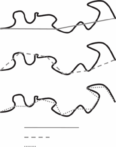
Consider the problem of estimating the fractal dimension of a convoluted line, such as a coastline,
vegetation patch edge, or movement pathway. Using the dividers procedure, the fractal dimension
D
d
is estimated by measuring the length of a curve at various scale values d (Figure 3.4). The pro-
cedure is analogous to moving a set of dividers (like a drawing compass) of xed length d along the
curve. The estimated length of the curve is the product of N(d ) (the number of compass dividers
A
B
C
δ
1
δ
2
δ
3
Figure 3.4 Schematic illustration of three successive steps of the divider procedure using dividers d
1
(A), d
2
(B),
and d
3
(C) of decreasing lengths.
2782.indb 29 9/11/09 12:03:33 PM
30 Fractals and Multifractals in Ecology and Aquatic Science
required to “cover” the object) and the scale factor d. The number of dividers necessary to cover
the object increases with decreasing measurement scale, leading to the power-law relationship:
L(d) = kd
m
(3.9)
where d is the measurement scale, L(d ) is the measured length of the curve, L(d ) = Nd, and k is
a constant. Practically, the fractal dimension D
d
is estimated from the slope m of the log-log plot
of L(d ) versus d for various values of d where:
D
d
= 1 − m (3.10)
One must note that, because L(d) = N(d )d, Equation (3.10) can be equivalently written as:
N(d) = kd
−D
d
(3.11)
The fractal dimension D
d
is then directly estimated from the slope of the log-log plot of N(d ) ver-
sus d. Note that the fractal properties of a curve have also been investigated using the mosaic tile
amalgamation method, or boundary method (Kaye 1989). In this method, a curve is covered by a
grid with each box having a length d, called the mosaic tile size, and the perimeter of the curve is
calculated for each tile size as the product of the number of boxes that intersect the curve and the
size of the box. By superimposing many different grid sizes, the perimeter of a curve is then given
by the scaling relationship (Kaye 1989):
P
D
b
∝
−
δ
1
(3.12)
where D
1b
is the boundary fractal dimension, and
means proportionality.
The fractal dimension D
d
is bounded between 1 and 2 when the curve is Euclidean and space ll-
ing, respectively. In the former case, the length of the curve is a constant independent of the length
scale d. This lower bound is nevertheless proven to be true only when d is sufciently small when
compared to the characteristic external scale of a given object. For instance, the perimeter of a circle
of radius r is constant when d = r. When D
d
= 2, the curve is so convoluted that it lls the whole
available (two-dimensional) space; the length of the curve is linearly related to d.
Even though coastlines, patch boundaries, and movement pathways are curves, their wiggli-
ness is so extreme that it is practically innite. For example, it is not useful to assume that they
have either well-dened tangents (Perrin 1913) or a well-dened nite length (Mandelbrot 1967).
Specic measures of the length depend on the method of measurement and have no intrinsic mean-
ing. For example, let a pair of dividers “walk” along the coast; as the step length d is decreased, the
number N(d ) of steps necessary to cover the coast increases faster than 1/d. Hence, the total distance
covered, L(d ) = N(d )d, increases without bound.
3.2.1.1.1 Divider Dimensions and the Length of Coastlines
The dividers method was originally used to describe the fractal nature of coastlines. From
Mandelbrot’s (1967) seminal paper “How Long Is the Coast of Britain? Statistical Self-Similarity
and Fractional Dimension,” chapters in standard monographs and textbooks on fractals (for exam-
ple, Feder 1988; Turcotte 1992) discussed the fractal nature of coastlines at length. Mandelbrot
(1983) examined a small set of coastlines and found their fractal dimension to be in the range of
1.2 to 1.3. Later work investigated the fractal dimension D
d
for a limited sample of other coastlines
(Dietler and Zhang 1992; Feder 1988; Carr and Benzer 1991; Pennycuick and Kline 1986; Korin
1992; Paar et al. 1997; Jiang and Plotnick 1998; Zhu et al. 2000, 2004) (see Table 3.1). For instance,
Jiang and Plotnick (1998) showed that the Atlantic coast of the United States was much more complex
2782.indb 30 9/11/09 12:03:35 PM

Self-Similar Fractals 31
than the Pacic coast. This is consistent with previous qualitative statements describing the Pacic
coast as being unique among the coastlines of the world in that the evenness of its contour is almost
unbroken by embayments (Keen 1971). In contrast, the Atlantic coast is extensively embayed, with
numerous fjords and river systems. In addition, no latitudinal gradient was detected in the fractal
dimensions estimated over 1° latitudinal ranges, although they signicantly increased from North
to South on the Atlantic coast. Hypothesizing that the spatial complexity of a coastline can be
regarded as a proxy of the bathymetric complexity of the related ocean oor, Jiang and Plotnick
(1998) suggested that the bathymetric complexity of the Atlantic Ocean oor adjacent to the United
States is far more complex than that of the corresponding Pacic Ocean oor. In an attempt to
assess the potential impact of the lithologic properties of faults on the development of the east coast
of Britain, Philip (1994) found that in some areas the coastlines were parallel to the faults. This
was later conrmed by a fractal analysis of the coastline of China showing both direct and indirect
effects of faults on coastline complexity (Zhu et al. 2004). Although the general trends of coast-
lines are forced by the geometry of the faults, the more active the faults are, the smaller the fractal
dimension of the coastline is (Zhu et al. 2004). The potential implications of the fractal nature of
coastlines (and ultimately of any potential habitat) on species diversity and species extinction are
discussed hereafter.
3.2.1.1.2 Coastline Complexity and Marine Species Diversity
Many explanations for diversity patterns have been proposed, and there have been several early
reviews of the subject (for example, Pianka 1966, 1974; Pielou 1975). High diversity has been attrib-
uted both to intense competition, which forces niche restriction (MacArthur and Wilson 1967;
Hutchinson and MacArthur 1959; MacArthur 1965), and reduced competition resulting from pre-
dation (Risch and Carroll 1986). However, along with a variety of ecological and evolutionary
processes, historical events, and geographical circumstances, habitat complexity on a wide range
of scales plays an important role in community structure (Schluter and Ricklefs 1993; Rahbek and
table 3.1
Fractal divider dimension D
d
of a range of coastlines
coastline D
d
sources
Adak Island, Alaska (USA) 1.20 Pennycuick & Kline (1986)
Amchitka Island, Alaska (USA) 1.66 Pennycuick & Kline (1986)
West Coast (Great Britain) 1.27 Carr & Benzer (1991)
North Coast (Australia) 1.19 Carr & Benzer (1991)
South Coast (Australia) 1.13 Carr & Benzer (1991)
West Shore, Puget Sound (USA) 1.19 Carr & Benzer (1991)
East Shore, Puget Sound (USA) 1.15 Carr & Benzer (1991)
West Shore, Gulf of California (USA) 1.03 Carr & Benzer (1991)
East Shore, Gulf of California (USA) 1.02 Carr & Benzer (1991)
Ria Coast from Kamaishi (Japan) 1.21–1.37 Korin (1992)
Louisiana (USA) 1.20 Lam & DeCola (1993)
Pacic Coast (USA) 1.00–1.27 Jiang & Plotnick (1998)
Pacic Coast (USA) 1.00–1.70 Jiang & Plotnick (1998)
Jiangsu Province (China) 1.07 Zhu et al. (2000)
Coastline of China 1.04–1.24 Zhu et al. (2004)
Van Koch Curve 1.21 Carr & Benzer (1991)
Fractal Brownian Coastline 1.30 Mandelbrot (1977)
2782.indb 31 9/11/09 12:03:36 PM
32 Fractals and Multifractals in Ecology and Aquatic Science
Graves 2001). Environmental heterogeneity is critical for species coexistence, with structurally
complex habitats offering a great variety of different microhabitats and niches, thereby allowing
species to coexist and contributing to within-habitat diversity (Pianka 1988). Habitat heterogeneity
provides a diversity of resources that can lead to coexistence of competitors, which would not be
possible in homogeneous environments (Levin 1992) and is, de facto, a critical mechanism in the
maintenance of biological diversity (Levin 1981). Although theoretical support for the importance
of habitat heterogeneity is overwhelming, empirical evidence is not always clear and can be con-
founding (Kareiva 1990). Many studies conducted in a variety of ecosystems thus support a positive
relationship between habitat complexity and species diversity (Petren and Case 1998; Kerr et al.
2001; Rahbek and Graves 2001), although evidence exists for diversity decreasing with or being
independent of habitat heterogeneity (Eadie and Keast 1984; Kelaher 2003; Taniguchi et al. 2003).
According to the above-mentioned statements, the increase in complexity of the Atlantic coast of the
United States identied by Jiang and Plotnick (1998) should favor a higher species diversity when
compared to the Pacic coast. Valentine (1989) identied 468 shallow-water gastropod species from
the Californian faunal province of the Pacic coast, while for similar latitudes in the Atlantic, Allmon
et al. (1993) found 778 gastropod species from the east coast of Florida. These results support the long-
standing hypothesis of a positive relationship between habitat complexity and species diversity, and the
potential for fractal analysis to be related with more traditional biological and ecological approaches
in entangling the complex relationship between habitat heterogeneity and species diversity.
3.2.1.1.3 Coastline Complexity and Species Extinction
A mass extinction of coastal marine mollusks along the Atlantic coast of the United States in the
late Pliocene has been well documented (Schopf 1970; Stanley 1981; Allmon et al. 1993); only
22% of Early Pliocene bivalve species have survived (Stanley 1986). In contrast, 80% and 75% of
the Pacic coast Pleistocene fossil species of bivalves and gastropods, respectively, are still living
(Valentine 1989). Stanley (1986) has suggested that the western Atlantic extinction was produced
by cooling associated with the onset of glaciation. The cooling of the Pacic was proposed to be
much weaker, so that no extinction resulted. However, an alternative explanation may lie in the
topographic changes related to sea-level drop and climate change (Jiang and Plotnick 1998). As
Valentine (1989) suggested, the early Pliocene coastline of the U.S. Atlantic coast was less com-
plex than that of today, so an increase in coastline complexity may have increased speciation rates,
resulting in the observed increase in diversity. Considering the observed higher complexity of the
coastlines of the Atlantic coast, it is likely that the sea-level changes related to climate forcing
induced sharper changes in the local properties of habitat complexity, which might have also con-
tributed to species extinction.
3.2.1.2 case study: movement Patterns of the ocean sunfish, Mola Mola
3.2.1.2.1 Study Organism
The ocean sunsh, Mola mola, inhabit tropical and temperate regions of the Mediterranean Sea and
the Atlantic, Indian, and Pacic oceans (Fraser-Brunner 1951; Wheeler 1969; Miller and Lea 1972).
Key aspects of their biology and behavior, such as annual movement and the mode and location
of breeding, are still largely unknown (Fraser-Brunner 1951; Reiger 1983). It has been suggested
that the main part of their life is spent in deep water (Fraser-Brunner 1951; Lee 1986); however,
ocean sunsh are frequently observed during daylight hours at the sea surface (Fraser-Brunner
1951; McCann 1961; Schwartz and Lindquist 1987; Sims and Southall 2002; Seuront et al. 2003). In
a recent study of their ne-scale movements, ocean sunsh were found to exhibit nocturnal vertical
movements within the surface mixed layer and thermocline, while diurnal vertical movements were
characterized by repeated dives below the thermocline (Cartamil and Lowe 2004). Although ocean
sunsh have been previously regarded as planktonic sh, primarily passively transported by oce-
anic currents (McCann 1961; Lee 1986), Cartamil and Lowe (2004) showed that ocean sunsh are
2782.indb 32 9/11/09 12:03:36 PM
Self-Similar Fractals 33
active swimmers not signicantly affected by the velocity or the direction of the currents, and with
cruising speeds similar to those found for yellown tuna Thunnus albacares (Block et al. 1992).
3.2.1.2.2 Experimental Procedures and Data Analysis
The data used here to investigate the diel variability of the ne-scale properties of ocean sunsh
movement patterns were originally described in a previous study (Cartamil and Lowe 2004). As a
consequence, we only provide hereafter the basics of capturing, tagging, and tracking procedures
(Figure 3.5) and refer the reader to Cartamil and Lowe (2004) for further details. Eight ocean sun-
sh were captured by dipnetting while basking at the surface or found in association with kelp pat-
ties, and measured and tagged with a temperature and depth-sensing acoustic transmitter (Vemco,
Model V22TP, 22 mm diameter × 100 mm length, frequencies 34 to 40 kHz). The acoustic output
of the transmitters was detected using a xed directional hydrophone mounted through the vessel’s
hull, and decoded by a receiver unit (Vemco, Model VR-60) mounted above the boat console (see
Cartamil and Lowe 2004 for more details). Depth, temperature, and GPS-derived location of the
vessel were recorded every 3 minutes.
Although the fractal nature of sh movement patterns have seldom been studied (Coughlin et al.
1992; Dowling et al. 2000; Faure et al. 2003), it may nevertheless be thought of as a unifying frame-
work to model and compare movement patterns of other groups of organisms (Turchin 1998; Faure
et al. 2003). Although movement patterns of ocean sunsh have been limited to scale-dependent
measurements, such as rate and directionality of movement, the same data used to determine these
metrics can be used to calculate and compare the fractal dimension of these movements (Cartamil
and Lowe 2004). The use of the dividers dimension D
d
is illustrated on the basis of acoustic telem-
etry tracking data for Mola mola off the southern California coast (Figure 3.6A) and demonstrates
the fractal nature of diurnal and nocturnal movement patterns (Figure 3.6B).
3.2.1.2.3 Results
For the eight trajectories considered, log-log plots of L(d ) versus d (Equation 3.9) exhibit very strong
linear behaviors over the whole range of considered scales, with coefcients of determination rang-
ing from 0.98 to 0.99 (Figure 3.6C). This unambiguously demonstrates the scale-dependent (fractal)
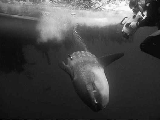
Figure 3.5 An ocean sunsh, Mola mola, released immediately after tagging with a temperature and depth-
sensing acoustic transmitter. (Courtesy of Dr. C. G. Lowe, California State University, Long Beach, California.)
2782.indb 33 9/11/09 12:03:37 PM