Seuront L. Fractals and Multifractals in Ecology and Aquatic Science

Подождите немного. Документ загружается.

34 Fractals and Multifractals in Ecology and Aquatic Science

nature of sunsh movement patterns. Although no differences were “visually” perceptible between

diurnal and nocturnal movement patterns, the resulting fractal dimensions, plotted as a function of

diurnal and nocturnal movement patterns for each individual’s swimming path, ranging from 1.05

to 1.31, show a high individual variability (Figure 3.6D). Except for the paths 5, 6, and 8, nocturnal

fractal dimensions were signicantly higher than diurnal ones (analysis of covariance and subse-

quent Tukey test, p < 0.01, Figure 3.6D). A signicant negative correlation ( p < 0.05) was found

between sunsh size and both diurnal and nocturnal fractal dimensions. A signicant ( p < 0.05)

positive correlation was found between nocturnal temperature and fractal dimensions. This relation

was nonsignicant ( p > 0.05) during daylight hours.

3.2.1.2.4 Ecological Interpretation

The difference between diurnal and nocturnal fractal dimensions suggests two specic swimming

strategies (Figure 3.6D). The relative linearity associated to the low fractal dimension during daylight

hours suggests individuals are moving in a direct manner. In contrast, the more complex, convoluted

Latitude

Longitude

Kilometers

0510

1.4

1.3

1.2

Fractal Dimension D

Log L (δ)

Log δ

Ocean Sunﬁsh

1.1

1.0

0.0

0.5

1.0

1.5

2.0

2.5

3.0

3.5

4.0

4.5

= 1.30

= 1.17

0.0

0.5

1.0

1.5

2.0

2.5

12345678

15 20

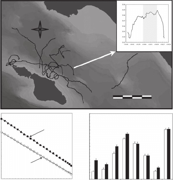
Figure 3.6 (A) Movements of eight ocean sunsh, Mola mola, tracked by acoustic telemetry, near Santa

Catalina Island, California. (B) Details of diurnal and nocturnal (shaded area) movement patterns for the indi-

viduals. (C) Illustrations of the related diurnal (open symbols) and nocturnal (black symbols) scaling behaviors

of the log-log plot of L(d ) versus d (see Equation 3.9). (D) Fractal dimensions D

are shown for the diurnal

(white bars) and nocturnal (black bars) movement patterns of the eight individuals.

2782.indb 34 9/11/09 12:03:40 PM

Self-Similar Fractals 35

paths observed during the nighttime period suggest that sunsh are interacting with environmental

heterogeneity on a ner scale (Wiens et al. 1995). As shown for a variety of organisms ranging from

minute invertebrates (Crist et al. 1992; With 1994; Hoddle 2003; Seuront 2006) to large mammals

(Bascompte and Vilà 1997; Ferguson et al. 1998a, 1998b; Mouillot and Viale 2001; Mårell et al.

2002; Laidre et al. 2004), an increase in the complexity of spatial movements may also indicate an

increase in foraging or searching efforts in a localized area. Therefore, this may suggest that sunsh

were searching for more clumped resources at night. Ocean sunsh vertical dive proles observed

during daylight hours may enable them to feed on vertically migrating gelatinous zooplankton at their

diurnal depths below the thermocline (Cartamil and Lowe 2004). Here, the higher fractal dimension

observed at night for ve of the eight ocean sunsh investigated might be related to an increased

foraging activity on gelatinous zooplankton occurring near the surface nocturnally. This result does

not contradict previous work suggesting that sunsh are feeding primarily during the day. Instead,

this may further substantiate the hypothesis that the movement patterns of ocean sunsh could have

evolved as a means of foraging on vertically migrating organisms, and previous observations of noc-

turnal vertical movements were conned to the surface layer and thermocline (Cartamil and Lowe

2004). Ocean sunsh may also be feeding during both day and night but use different movement

patterns to fully exploit prey that vertically migrate. The potential link between environmental het-

erogeneity and sunsh behavior was previously investigated by looking at sunsh movements relative

to sea-surface temperature fronts (Cartamil 2003). However, the cloud cover that limited sea-surface

temperature image quality and availability over the study area hampered the identication of any

relationship (Cartamil 2003). The observed changes in fractal dimensions of swimming trajectories

may then provide an efcient, alternative tool to infer changes in environmental properties.

The signicant negative correlation between ocean sunsh size and the fractal dimension

(p < 0.05) of their swimming paths suggests that larger individuals interact with their environment

at a ner scale resolution than do smaller ones. Assuming that larger sunsh have increased remote

sensing ability and motility, they may achieve more convoluted (that is, high D value) swimming

paths, likely to increase their encounter rates with their intrinsically patchy zooplankton prey. A

more convoluted swimming strategy also increases predation risk (see, for example, Tiselius et al.

1997), and ocean sunsh are typically hunted by fast-swimming predators such as large sharks

(Fergusson et al. 2000) and California sea lions (Cartamil and Lowe 2004). However, since preda-

tion risk is less likely at large sizes, their size may enable them to use this type of movement rela-

tively safely. In contrast, the more linear swimming behavior of the smallest and slowest sunsh

(that is,

D 1.14 0.01;=± ±x SD

) could then be thought as an antipredator strategy.

The signicant positive correlation between temperature and the tortuosity of nighttime move-

ment patterns suggests that the foraging activity of ocean sunsh may be temperature dependent.

This may be directly related to an increased motility in warmer waters but also to different foraging

strategies. This is consistent with the high individual variability observed in the movement patterns

(Figure 3.6D) as different individuals moved over similar areas (see Figure 3.6A) but at different

times. These areas likely differed in their biotic and abiotic properties during each tracking period.

In particular, studies have documented the hierarchical nature of marine species’ responses to food

patch structure (Fauchald et al. 2000), indicating that organisms may be specically responding to

different prey distribution or density (Seuront et al. 2001).

3.2.1.3 methodological considerations

3.2.1.3.1 How to Start the Analysis?

As illustrated in Figure 3.4, the implicit easiest way to conduct the analysis is to use the rst point

of the object under consideration as a starting point for the divider algorithm. However, the val-

ues L(d ) = Nd may vary depending on the starting position along the curve, especially at large

scales (Sugihara and May 1990a; With 1994; Nams 1996). This issue can nevertheless be circum-

vented by starting the dividers procedure at different, randomly chosen positions, walking forwards

and backwards, and using the distribution of the resulting divider dimensions (also referred to as

2782.indb 35 9/11/09 12:03:41 PM

36 Fractals and Multifractals in Ecology and Aquatic Science

“compass dimension” in the literature) as an estimate of D

. This procedure has been applied on

nine three-dimensional swimming paths of the freshwater crustacean, the water ea Daphnia pulex

(see Figure 3.12). Taking 10 random starting positions for each of the swimming paths available,

Seuront et al. (2004a) did not identify any spurious effect related to the rst point considered in the

analysis, as all the divider dimensions returned were not found signicantly different (analysis of

covariance, p > 0.05). It is strongly advised, however, to systematically infer this potential bias to

ensure the relevance of the divider dimension returned by the analysis.

3.2.1.3.2 On the Relevance of Fractal Analysis in Movement Ecology

3.2.1.3.2.1 Fractal Analysis in Movement Ecology

Since its introduction to characterize tortuosity of animal trails (Dicke and Burrough 1988), frac-

tal analysis has been widely used to describe movement pathways of a wide variety of organisms

ranging from invertebrates to large vertebrates (Table 3.2). The fractal analysis of animals’ paths

appeared to be an alternative and promising method for measuring tortuosity of foraging behavior.

Although D

is primarily a measure of the extent to which a given (fractal) object lls the space in

which it is embedded, the logic of the use of fractals to characterize motion behavior lies behind

table 3.2

nonexhaustive literature survey of movement Pathways analyzed using Fractal

dimensions

organism terrestrial aquatic sources

Vertebrate

Cody (1971)

Invertebrate*

Shlesinger (1986)

Invertebrate + Dicke & Burrough (1988)

Invertebrate*

Levandowski et al. (1988)

Invertebrate

Wiens & Milne (1989)

Invertebrate

Turchin et al. (1991)

Invertebrate

Crist et al. (1992)

Invertebrate

Johnson et al. (1992)

Invertebrate

Coughlin et al. (1992)

Invertebrate

Bundy et al. (1993)

Invertebrate

Gautestad & Mysterud (1993)

Invertebrate

With (1994)

Invertebrate

Erlandson & Kostylev (1995)

Invertebrate

Wiens et al. (1995)

Invertebrate

Cole (1995)

Invertebrate

Brewer (1996)

Vertebrate*

Viswanathan et al. (1996)

Invertebrate*

Schuster & Levandowsky (1996)

Vertebrate

Nams (1996)

Vertebrate*

Focardi et al. (1996)

Invertebrate

Turchin (1996)

Invertebrate

Jonsson & Johansson (1997)

Vertebrate*

Kafetsopoulos et al. (1997)

Vertebrate

Bascompte & Vila (1997)

Invertebrate

Turchin (1998)

Vertebrate

Ferguson et al. (1998a)

Vertebrate

Ferguson et al. (1998b)

Vertebrate

Etzenhouser et al. (1998)

Vertebrate

Dowling et al. (2000)

2782.indb 36 9/11/09 12:03:42 PM

Self-Similar Fractals 37

the two extreme representations of organism movement. The rst extreme is an organism mov-

ing along a perfectly linear path. As previously described, since the path is a line, its length L(d )

will always be the same whatever the measurement scale d (that is, the size of the divider) and its

fractal dimension is unity. The second extreme is the Brownian motion, which results in a fractal

dimension D

= 2, suggesting that all points in the available space have been visited, leaving no

area unlled. The fractal dimension is then expected to provide a measure of the path sinuosity or

tortuosity. However, the critique made by Turchin (1996), and to a lesser extent Benhamou (2004),

might throw some doubt on the reliability of the fractal dimension for measuring organisms’ path

tortuosity. The advantages of using fractal analysis instead of more traditional behavioral metrics

and the rationale for criticism against the fractal approach in behavioral ecology are addressed in

details hereafter.

3.2.1.3.2.2 Scale Independence or Scale Dependence of Fractal Dimension of Movement

Pathways?

The key assumption of fractal analysis is that the fractal dimension is scale independent; that is,

the fractal dimension estimated from a movement path that is tens of meters long is the same for

paths measured at the scale of meters to kilometers. This is not the case, however, for traditional

behavioral metrics (Box 3.1).

Invertebrate

Schmitt & Seuront (2001)

Vertebrate

Mouillot & Viale (2001)

Vertebrate*

Marell et al. (2002)

Vertebrate*

Atkinson et al. (2002)

Vertebrate

Fritz et al. (2003)

Invertebrate

Hoddle (2003)

Invertebrate*

Bartumeus et al. (2003)

Vertebrate

Laidre et al. (2004)

Vertebrate

Faure et al. (2003)

Invertebrate

Martin (2004)

Vertebrate*

Austin et al. (2004)

Invertebrate

Seuront et al. (2004a)

Invertebrate

Seuront et al. (2004b)

Invertebrate

Seuront et al. (2004c)

Vertebrate*

Ramos-Fernández et al. (2004)

Invertebrate

Biesinger & Haefner (2005)

Vertebrate

Nams (2005)

Vertebrate

Garcia et al. (2005)

Invertebrate

Uttieri et al. (2005)

Invertebrate

Uttieri et al. (2007)

Invertebrate

Seuront (2006)

Invertebrate*

Reynolds (2006)

Invertebrate*

Reynolds & Frye (2007)

Invertebrate*

Reynolds et al. (2007)

Invertebrate*

Seuront et al. (2007)

Vertebrate**

Bertrand et al. (2007)

Vertebrate**

Brown et al. (2007)

Vert/Invert*

+ +

Edwards et al. (2007)

Vertebrate* + Sims et al. (2008)

*Movement pathways analyzed indirectly as Lévy ights using cumulative frequency distributions, see Chapter 5.

**Humans.

2782.indb 37 9/11/09 12:03:43 PM

38 Fractals and Multifractals in Ecology and Aquatic Science

Box 3.1 on thE SCALE DEPEnDEnCE oF

tRADItIonAL BEhAvIoRAL MEtRICS

Movement pathways have been characterized by a variety of measures, including path length

(the total distance traveled, or gross displacement), move length (the distance traveled between

consecutive points in time), move duration (time interval between successive pauses, as well

as between successive spatial points), speed (move length divided by move duration), turning

angle (the difference in direction between two successive moves), turning rate (turning angle

divided by move duration), net displacement (the linear distance between starting and ending

points, often used as a metric when making comparisons with diffusion or correlated ran-

dom walk models; see, for example, Kareiva and Shigesada 1983; McCulloch and Cain 1989;

Turchin 1991; Johnson et al. 1992), and NGDR (net to gross displacement ratio; Wilson and

Greaves 1979). As discussed by Seuront et al. (2004a), the values of all the metrics are implic-

itly a function of their measurement scale. The scale dependence of these ratio metrics—that

is, the path length and the turning angle (Figure 3.B1.1)—implies that there is no single scale

at which movement paths can be unambiguously described.

Figure 3.b1.1 Illustration of the scale dependence of path length (A) and turning angle (B) of the

swimming trajectories of the water ea, Daphnia pulex, investigated at different temporal resolution

and spatial scale, respectively. (Modied from Seuront et al., 2004a.)

Path Length (cm)Turning Angle (rad)

1.0

0.9

0.8

0.7

0.6

12 43

Time Scale (s)

Spatial Scale (cm)

5678910 11

0.0 0.3 0.6 0.9 1.2 1.5 1.8 2.1

y = 46.30 – 15.09 log x

r = 0.98

2782.indb 38 9/11/09 12:03:45 PM

Self-Similar Fractals 39

Scale measurement is the central tenet of one of the main issues faced by landscape ecolo-

gists: understanding how to meaningfully extrapolate ecological information across spatial scales

(Gardner et al. 1989; Turner and Gardner 1991). The scale independence of the fractal dimension

is mainly driven by the belief that the same process is controlling the observed patterns from the

smallest to the largest available scales. Strictly speaking, fractals are mathematical constructs

characterized by a never-ending cascade of similar structural details that are revealed upon mag-

nication on all scales. A fractal object, considered in its mathematical sense, then requires

“many” orders of magnitude of power-law scaling, and subsequent interpretation of empirical

data as indicating fractality must require “many” orders of magnitude (Avnir et al. 1997). While

the concept of “many orders of magnitude” might be thought of as fairly vague in itself, it refers

to several key processes involving equilibrium-critical phenomena (such as magnets, liquids,

percolations, and phase transitions) and some nonequilibrium growth models (such as diffusion-

limited aggregation, stopovers of Lévy ights) that are backed by intrinsically scale-free theories

and lead therefore to power-law scaling behavior on all scales. It is then legitimate to expect con-

stant fractal dimensions over up to ve decades (Avnir et al. 1997). This is, however, very unlikely

to happen in ecology due to the heterogeneous and hierarchical organization of landscapes and

ecosystems.

Wiens et al. (1993) concluded their investigation of insect movement in microlandscape mosa-

ics, stating that “because the fractal dimension has the desirable feature of being constant over

a nite range of measurement scales, it is useful in comparing movements of insects that may

respond to the patch structure of the environment at different absolute scales.” A fractal motion

behavior is also implicitly limited by the sizes of the organisms and their home range, or more

prosaically by the size of the enclosure in which their behavior has been investigated. These

potential changes in fractal dimensions then dene transitions between different spatial domains

for which the fractal dimension is scale independent (Wiens 1989). As a consequence, the fractal

dimensions of organisms’ movements are expected to apply to a limited range of scales or to

change with scales (Box 3.2).

Box 3.2 on thE SCALE InDEPEnDEnCE oF FRACtAL

DIMEnSIonS In AnIMAL BEhAvIoR

The traditional dividers method (Section 3.2.1.1) can be adapted to measure D

over dif-

ferent ranges of scales (Krummel et al. 1987; Sugihara and May 1990a; Nams 1996). First,

consider a regression window varying over a range of divider lengths d (where a minimum

of ve values is expected to ensure the statistical relevance of a regression analysis; Seuront

et al. 2004a), and estimate the slope of the log-log plot of L(d ) vs. d over that range, thus the

fractal dimension D

. Then shift the range of the d value along the x axis, and estimate D

again. This procedure is illustrated using swimming paths of adult males and females of the

subtropical copepod, Oncaea venusta (Figure 3.B2.1), which have been investigated using the

dividers method (Section 3.2.1.1) and the sliding regression-window method described above

(Figure 3.B2.2).

The very strong linear behavior of log-log plot of L(d ) vs. d for the male trajectory

over more than two decades (Figure 3.B2.2A) and the lack of variability in the fractal

dimension D

obtained from the sliding regression-window procedure (Figure 3.B2.2C)

suggest the fractal character of the motion behavior of O. venusta. Similarly, the female

swimming path clearly exhibits two distinct scaling behaviors below and above a critical

scale of 10 mm (Figure 3.B2.2B), which have been confirmed by the sliding window

2782.indb 39 9/11/09 12:03:46 PM

40 Fractals and Multifractals in Ecology and Aquatic Science

regression procedure (Figure 3.B2.2D). As the identied behaviors signicantly differed from

a correlated random walk model ( p < 0.05; see the procedure described in Box 3.3), it is legiti-

mate to conclude the fractal character of the movement pathways of both male and female O.

venusta.

Because different scales are often associated with different driving processes, the fractal

dimension may have the desirable feature of only being constant over a nite, instead of

an innite, range of measurement scales. It is then useful for (1) identifying characteristic

scales of variability, and (2) comparing movements of organisms that may respond, for

instance, to the patchy structure of their environment at different absolute scales. Changes

in the value of the fractal dimension with scale may indicate that a new set of environmental

or behavioral processes is controlling movement behavior (for example, decreased inuence

of patch barriers or the effect of home-range behavior). Thus, the scale dependence of the

fractal dimension over nite ranges of scales may carry more information, both in terms of

driving processes and sampling limitation, than its scale independence over a hypothetical

innite range of scales. Alternatively, although the point of slope change may indicate the

operational scale of different generative processes, it may simply reect the limited spatial

resolution of the data being analyzed (Kenkel and Walker 1993; Gautestad and Mysterud

1993). However, discussed elsewhere (Seuront et al. 2004a), the effect of spatial resolution

in the data will manifest itself as a gradual change of the fractal dimensions toward

→1

→2,

and cannot be confused with a transition zone between two different scaling

regions as illustrated here.

In order to measure if—and then eventually how and why—organisms use habitats at different

scales, it is critical not only to measure the overall fractal dimension but also to measure how the

fractal dimension changes with scale. The signatures of the log-log plot of L(d ) vs. d returned by

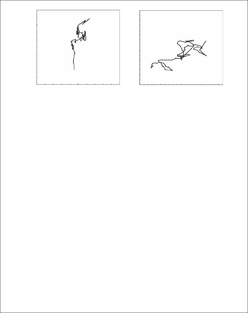
Figure 3.b2.1 Examples of swimming paths of adult female (A) and male (B) of the subtropical

copepod, Oncaea venusta.

0510

X (cm)

2015

Y (cm)

510

X (cm)

Y (cm)

2782.indb 40 9/11/09 12:03:49 PM

Self-Similar Fractals 41

the swimming paths of ocean sunsh (Figure 3.6) and the subtropical copepod, Oncaea venusta

(Figure 3.B2.2A), typically spanning more than two decades and satisfying objective optimization

criteria (see Chapter 7), can then reliably be considered as fractal and exhibit the same move-

ment pattern over the whole range of available scales. In contrast, the two distinct movement pat-

terns observed in the female of the copepod, Oncaea venusta, above and below 10 mm (Box 3.2)

reveal two distinct foraging strategies over two distinct ranges of scales. Similar results have been

reported for the American marten (Martes americana), which displayed different responses to

their environment at scales smaller and greater than 3.5 m (Nams and Bourgeois 2004). At scales

smaller than 3.5 m, marten moved in a more direct way (that is, at a lower fractal dimension D

)

than at larger scales, suggesting different habitat use. This is consistent with earlier work by

Benhamou (1990), who showed that at a smaller scale wood mice (Apodemus sylvaticus) travel

in a directed path toward individual bushes, but at a larger scale they move from bush to bush

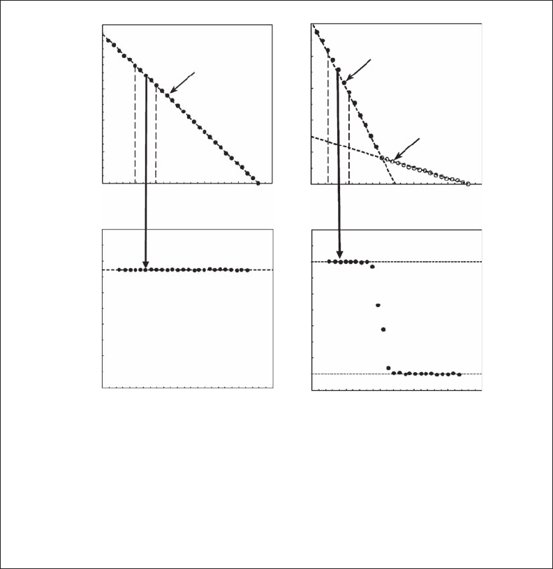
Figure 3.b2.2 Illustration of the “traditional” log-log plots of L(d) vs. d showing (A) the unique

scaling behavior of the swimming path of an adult male for scales ranging from 1.2 to 200 mm

= 1.37; A), and (B) the two distinct scaling behaviors of the swimming path of an adult female

for scales ranging from 1.2 to 10 mm (D

= 1.40) and from 10 to 200 mm (D

= 1.05; B). The fractal

dimension D

calculated from the plots (A) and (B) using a sliding window of ve points along the x

axis clearly conrms the results of the divider method. The dashed gray lines in (A) and (B) identify

the limits of the regression window, and the gray arrow indicates the related fractal dimension D

estimate.

= 1.37 (r

= 0.99)

= 1.40 (r

= 0.99)

= 1.05 (r

= 0.99)

1.0

0.8

0.6

0.4

0.2

0.0

1.5

1.4

1.3

1.2

1.1

1.0

1.5

1.4

1.3

1.2

1.1

1.0

0.5

0.4

0.3

0.2

0.1

0.0

Log δ

Log L (δ)

Log δ

0.0 0.5 1.0 1.5 2.0 2.5

2782.indb 41 9/11/09 12:03:52 PM

42 Fractals and Multifractals in Ecology and Aquatic Science

randomly. At the smaller scale, the directed path would show a constant D

, but at the larger

scale the correlated random walk would show an increasing D

. What is critical for a proper

interpretation of fractal dimensions is then the identication of the range of scales over which a

fractal dimension is invariant, as shown here for the ocean sunsh (Mola mola) and the copepod

(Oncaea venusta).

However, changes in fractal dimensions are not always as clear as the one observed for O.

venusta (Box 3.2) (Figure 3.B2.2D). Instead, the fractal dimension can smoothly change with

scales as observed for the wandering albatrosses (Fritz et al. 2003) (Figure 3.7A) and the American

marten (Nams and Bourgeois 2004) (Figure 3.7B). The limits of the transition scales have been

dened as the rst signicant break in the slope of the relationship between the path length and

the divider length (Nams 1996; Fritz et al. 2003; Nams and Bourgeois 2004). Transition scales

are then centered on a minimum or maximum fractal dimension, with the surrounding dimen-

sions gradually increasing or decreasing (Figure 3.7). The above-mentioned denition of transi-

tion scales should consequently be rened as “the transition between different spatial domains

for which the fractal dimension is changing continuously with scale.” Using this concept allowed

Fritz et al. (2003) to identify a consistent pattern in the foraging paths of wandering albatrosses

(Diomedea exulans) over scales ranging across ve orders of magnitude (10 m to 1000 km). The

11 birds considered thus consistently adjust the tortuosity of their paths to different environmental

1.3

1.2

1.1

1.03

1.02

1.01

1234567891020

0.01

Spatial Scale (km)

Spatial Scale (m)

0.1 110

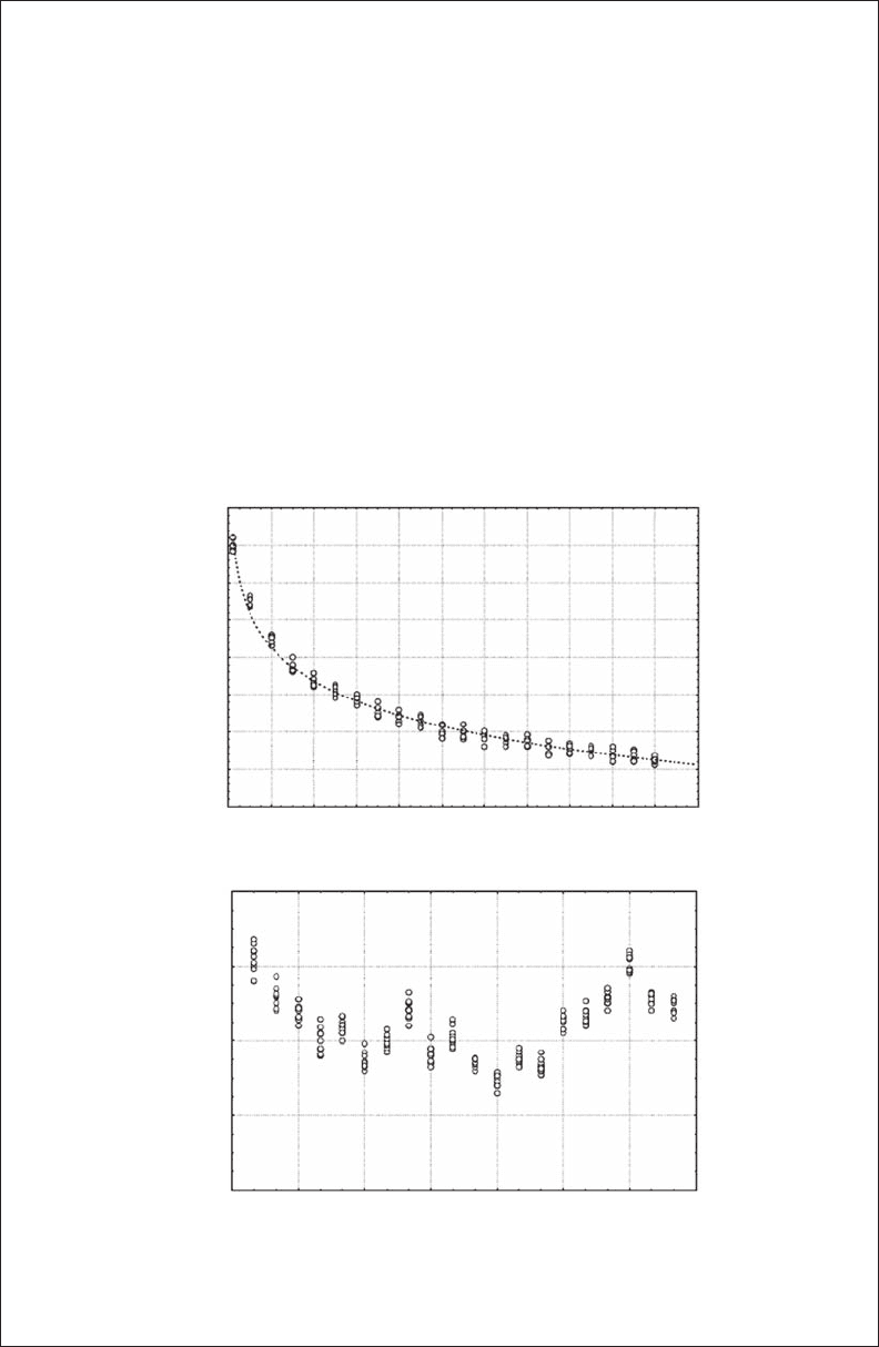
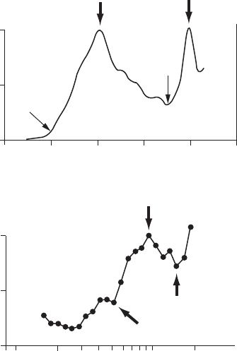
Figure 3.7 Patterns of the fractal dimension D

estimated at different spatial scales (that is, divider length d)

using the method described in Box 3.2, and used to identify transition scales in the movement pathways of (A)

wandering albatrosses (Diomedea exulans) (modied from Fritz et al. 2003); and (B) the American marten

(Martes americana) (modied from Nams and Bourgeois 2004). The transition scales originally chosen by the

authors are indicated by the thick arrows, and the question marks and thin arrows indicate additional transi-

tion scales that might also have been chosen given the shape of the relationship between D

and the spatial

scale and the denition found in Nams (1996), Fritz et al. (2003), and Nams and Bourgeois (2004).

2782.indb 42 9/11/09 12:03:53 PM

Self-Similar Fractals 43

and behavioral constraints over three distinct scale-dependent nested domains. At small scales,

they exhibit a zigzag movement to adjust for optimal use of wind; at intermediate scales, the

movement shows changes in tortuosity consistent with food-searching behavior; and at a large

scale, the movement relates to commuting between patches and to large-scale weather systems.

The absence of such transitions in sunsh trajectories implies that they were using the same for-

aging strategies over the whole range of scales considered. It is nevertheless acknowledged that

the choice of transition scales can sometimes seem fairly arbitrary (Figure 3.8) (see also Fritz et al.

2003, Figure 2A), stressing the need to use objective, statistically sound procedures to ensure

the relevance of the measured fractal dimensions and transitions scales. The uses, misuses, and

abuses of fractal analysis that may lead to spurious results and conclusions are addressed in detail

in Chapter 6.

3.2.1.3.2.3 Movement Pathways, Correlated Random Walks, and Fractal Analysis

An alternative hypothesis is that “the fractal dimension is not constant but changes continuously

with scales” (Turchin 1996). Turchin (1996) suggested that if an organism moves according to a cor-

related random walk (Box 3.3), then fractal analysis of that movement is not justied.

Log L (δ )

Log δ

m = 0.30 (r

= 1)

m = 0.32 (r

= 0.97)

3.10

0.15B

0.05

–0.05

–0.15

0 0.1 0.2 0.3 0.4 0.5

10 100

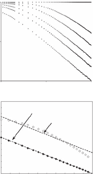
Figure 3.8 Inuence of the mean cosine of turning angles c (c = 0.0, 0.4, 0.6, 0.8, 0.9, and 1.0 from bottom

to top) (modied from Benhamou, 2004) of a simulated correlated random walk on the log-log plot of L(d ) vs.

d (A); and (B) illustration of the r

values returned by the power-law

L()

δδ



−03

(black symbols) and a sur-

rogate slightly nonlinear curve (open symbols).

2782.indb 43 9/11/09 12:03:56 PM