Seuront L. Fractals and Multifractals in Ecology and Aquatic Science

154 Fractals and Multifractals in Ecology and Aquatic Science

Sugihara and May (1990a) discussed its general relevance for a variety of different systems, ranging

from remote sensing to patch dynamics of bryozoans and coral colonies. In particular, they showed

the relationship between the Korcak dimension D

and the exponent H characterizing fractional

Brownian motions (Sugihara and May 1990a) (see also Chapter 4):

= 2 − H (5.11)

where H characterized the degree of persistence (or autocorrelation) of a pattern: For H < 0.5

and H > 0.5, a pattern is respectively negatively and positively autocorrelated, while H = 0.5 cor-

responds to the Brownian (that is, random) case (see Chapter 4 for further details). Sugihara and

May (1990a) additionally stated that increased persistence (more memory in the process) should

correspond to smoother boundaries and patches with larger and more uniform areas, whereas

reduced persistence will correspond to more complex and highly fragmented landscapes domi-

nated by many small areas.

5.4 Fragmentation and mass-size dimensions, D

and D

The Rosin law, widely used to describe the distribution of particle size in soils and other geologi-

cal material (Turcotte 1992), can be regarded as the volumetric analogy to the Korcak patchiness

exponent (Equation 5.9) and is dened as:

N(R ≥ r) = kR

−D

(5.12)

where k is a constant, N(R ≥ r) is the number of particles whose radius R is greater than a thresh-

old radius r, and D

is referred to as the fragmentation dimension, and condenses the information

about the scale dependence of the number-size distribution of soil aggregates (Turcotte 1986, 1989;

Perfect and Kay 1991; Perfect et al. 1992; Rasiah et al. 1992). A soil with a high fragmentation

dimension is then more fragmented and dominated by small particles, while D

= 0 is indicative of

a homogeneous soil where all particles are of equal diameter.

However, counting the total number of aggregates of a given size is not always possible, espe-

cially for smallest sizes. This inconvenience can be avoided by inferring the number-size distribu-

tion from the mass-size distribution function M(x < X) of the cumulative mass of aggregates of

characteristic size less than X as (Perfect et al. 1992; Rasiah et al. 1993; Kozac et al. 1996):

M(x < X) = kX

(5.13)

where k is a constant, x is the aggregate size, and D

is the so-called mass-size dimension. The

relationship between the fragmentation dimension D

and the mass-size dimension D

is given by

(Tyler and Wheatcraft 1992):

= 3 − D

(5.14)

The fractal structure of soil aggregates has also been investigated following (Perfect et al. 1994):

N(X ≥ x

) = kx

−D

(5.15)

where x

is a normalized measure of aggregate size (for example, sieve aperture divided by aperture

of the largest sieve), N(X ≥ x

) is the cumulative number of fragments with normalized length X ≥ x

and k is the number of fragments not passing the largest sieve. Note that Equation (5.15) is strictly

equivalent to the size distribution of fragments resulting from a fractal reduction of a Euclidean

initiator (Mandelbrot 1983; Turcotte 1986) and to the Rosin law; see Equation (5.12).

2782.indb 154 9/11/09 12:10:43 PM

Frequency Distribution Dimensions 155

5.5 ranK-Frequency dimension, D

5.5.1 Zi p F ’s la w , hu m a n co m m u n i c aT i o n , a n d T h E pr i n c i p l E o F lE a s T EF F o r T

One of the most surprising instances of power laws is probably Zipf’s law, named after the Harvard

linguistic professor G. K. Zipf (1902–1950), which is the observation of frequency of occurrence of

any event as a function of the rank r, when the rank is determined by the above frequency of occur-

rence (that is, from n events, the most and least frequent ones will then have ranks r = 1 and r = n,

respectively). More specically, the Zipf law states that the frequency f

of the rth largest occur-

rence of the event is inversely proportional to its rank r as:

(5.16)

where f

is the frequency of the most frequent event in the distribution. Zipf’s law emerges from

almost all languages’ letters and words as an approximate slope of −1 in log-log plots of f

vs. r,

a result Zipf (1949) stated due to the “Principle of Least Effort” in communication systems, rep-

resenting a balance between the repetition desired by the listener and the diversity desired by the

transmitter.

Zipf’s law is based on what Zipf (1949) termed the “Principle of Least Effort” in which he pro-

poses that human speech and language are structured optimally as a result of two opposing forces:

unication and diversication. If a repertoire is too unied or repetitive, a message is represented

by only a few signals, and therefore less communication complexity is conveyed. Alternatively, if

a repertoire is too diverse or randomly distributed, the same message can be overrepresented by a

multitude of signals and, again, less communication is conveyed. These two opposite forces result in

a balance between unication and diversication. Zipf’s Principle of Least Effort can be statistically

represented by regressing the log of the frequency of occurrence of some event (that is, letters, char-

acters, words, morphemes, phonemes) as a function of the rank, where the rank is determined by

the above-mentioned frequency of occurrence. The balance between unication and diversication

leads to a power-law function with a slope close to unity. Zipf subsequently showed that a multitude

of diverse human languages (for example, English words, Nootka varimorphs and morphemes,

Plains Cree holophrases, Dakota words, German stem forms, Chinese characters, Gothic root mor-

phemes and words, Aelfric’s Old English morphemes and words, English writers from Old English

to Present, Old and Middle High German and Yiddish sources, and Norwegian writings), whether

letters, written words, phonemes, or spoken words, followed this principle and the predicted slope

of ca. −1.00. This balance has also been found in the study of manuscripts of unknown origin

such as the Voynich manuscript* (see, for example, Landini 2001; Schinner 2007) and optimizes

the amount of potential communication that can be carried through a channel from speaker to

receiver or from writer to reader. The structure of the system is thus neither too repetitive (the

extreme would be one signal for all messages) nor too diverse (the extreme would be a new signal

for each message, and in practice a randomly distributed repertoire would represent the highest

degree of diversity). A system exhibiting such a balance (that is, a –1.00 slope in a log-log plot of

frequency of occurrence vs. rank) can be thought to have a high potential capacity for transfer-

ring information, and as such has a high communication capacity. Note, however, that it only has

the potential to carry a high degree of communication, because Zipf’s statistic only examines the

structural complexity of the repertoire, not how the composition is internally organized within

the repertoire.

The Voynich manuscript is a 16th-century manuscript written in an unknown language and alphabet.

2782.indb 155 9/11/09 12:10:45 PM

156 Fractals and Multifractals in Ecology and Aquatic Science

5.5.2 Zi p F ’s la w , in F o r m a T i o n , a n d En T r o p y

Information theory (Shannon 1948, 1951; Shannon and Weaver 1949), although originally illus-

trated using statistically signicant samples of human language, generally provides quantitative

tools to assess and compare communication systems across species. Specically, this theory has

been applied to a wide range of animal communicative processes or sequential behavior (for exam-

ple, MacKay 1972; Slater 1973; Bradbury and Vehrencamp 1998). These include aggressive displays

of hermit crabs (Hazlett and Bossert 1965), aggressive communication in shrimp (Dingle 1969),

intermale grasshopper communication (Steinberg and Conant 1974), dragony larvae communica-

tion (Rowe and Harvey 1985), social communication of macaque (Altmann 1965), waggle dance

of honeybees (Haldane and Spurway 1954), chemical paths of re ants (Wilson 1962), structure of

songs in cardinals and wood pewees (Chateld and Lemon 1970), vocal recognition in Mexican

free-tailed bats (Beecher 1989), and bottlenose dolphin whistles (McCowan et al. 1999). In contrast,

only few investigations have assessed animal behavior using Zipf’s law (Hailman et al. 1985, 1987;

Hailman and Ficken 1986; Ficken et al. 1994; Hailman 1994). The Zipf law and Shannon entropy*

are conceptually and mathematically related but nevertheless subtly differ. Zipf’s law measures

the potential capacity for information transfer at the repertoire level by examining the “optimal”

amount of diversity and redundancy necessary for communication transfer across a “noisy” channel

(that is, all complex audio signals will require some redundancy). In comparison, Shannon entro-

pies were originally developed to measure channel capacity, and the rst-order entropy differs from

Zipf’s statistic as Zipf does not specically recognize language as a noisy channel.

Both the similarity and difference between Zipf’s law and Shannon entropy prompted Mandelbrot

(1953) to analyze the question of how the value of the Zipf exponent a relates to the Shannon entropy†

(Equation 5.20; see also Box 5.1) for an information source following a Zipf’s distribution.

The main problem here is that the maximum rank is intrinsically controlled by the length of the

data set—that is, the vocabulary or repertoire size, or the number of species. In theory, the maxi-

mum rank can grow to innity. In practice, however, the maximum rank is limited to a nite value

Here, Shannon entropy specically refers to the rst-order Shannon entropy; Shannon higher-order entropies provide a

more complex examination of communicative repertoires and are discussed and illustrated in Section 5.5.6.

†

Note that entropy is dened here as a measure of the informational degree of organization and is not directly related to

the thermodynamic property used in physics; see also Box 5.1.

Box 5.1 thERMoDynAMIC EntRoPy

In scientic elds such as information theory, mathematics, and physics, entropy is generally

considered as a measure of the disorder of a system. More specically, in thermodynam-

ics (the branch of physics dealing with the conversion of heat energy into different forms

of energy—for example, mechanical or chemical), entropy, S, is a measure of the amount of

energy in a system that cannot be used to do work. Entropy can also be seen as a measure of

the uniformity of the distribution of energy. Central to the concept of entropy is the second

law of thermodynamics, which states that “the entropy of an isolated system which is not in

equilibrium will tend to increase over time, approaching a maximum value at equilibrium.”

Ice melting illustrated in Figure 5.B1.1 is the archetypical example of entropy increase

through time. First, consider the glass containing ice blocks as our system. As time elapses,

the heat energy from the surrounding room will be continuously transferred to the system.

Ice will then continuously melt until it reaches the liquid state, and the liquid will then keep

receiving heat energy until it reaches thermal equilibrium with the room. Through this pro-

cess, energy has become more dispersed and spread out in the system at equilibrium than

when the glass was only containing ice.

2782.indb 156 9/11/09 12:10:46 PM

Frequency Distribution Dimensions 157

due to nite sample size. This limitation, referred to as “rank truncation,” is at the core of the link

between a and H

(Figure 5.5):

The entropy of a Zipf’s distribution cannot be dened for • a ≥ −1 because the sum of all

probabilities is an innite series

∑

=r 1

∞

p(r), where p(r) = cr

, that diverges (Figure 5.5). In

contrast, for the region a < −1, where a ≈ −1, H

changes sharply with a. H

is then much

A striking property of entropy, the arrow of time, coined in the seminar work of the Nobel

laureate Ilia Prigogine, is implicit in the second law of thermodynamics. As the entropy of an

isolated system naturally tends to increase over time, it cannot decrease. This gives to ther-

modynamic processes a temporal directionality and irreversibility, especially clear from the

case of ice melting (Figure 5.B1.1).

Figure 5.b1.1 Ice melting as an example of entropy increase over time.

ABC

Shannon entropy

(bit)

Entropy sensitive

to rank truncation

Entropy insensitive

to rank truncation

Rank extend to inﬁnity

Rank up to p

α = –1

log

(p)

1/2

log

Entropy not

deﬁned unless

rank truncates

Figure 5.5 Shannon entropy H

shown as a function of the Zipf’s exponent a. The solid curve is the theo-

retical case where the rank r as no upper bound, that is, r → ∞. The dashed curve is the “rank truncation” case

that is practically encountered. (Modied from Mandelbrot, 1953.)

2782.indb 157 9/11/09 12:10:52 PM

158 Fractals and Multifractals in Ecology and Aquatic Science

more sensitive than a to a change in the source properties. As a consequence, two infor-

mation sources with very different values of H

will have similar values of a. a is thus a

poor parameter to characterize the communicative properties of information sources.

Rank truncation distorts entropy estimates in the region • a ≈ −1, which is also the region of

greatest interest for information sources close to the Zipf law (see Equation 5.16). Considering

the rank r of the least frequent word, Mandelbrot (1953) identied two cases where H esti-

mates are erroneously nite; that is, H

= log

r when a = 0 (the case where words are uni-

formly distributed) and H

= log

+ log

log

r when a = 1.

As a consequence, while both Zipf’s law and Shannon entropy directly relate to information theory,

this suggests that the Zipf distribution parameter a is a less reliable estimate and a less reliable rep-

resentation of the source properties than Shannon entropy.

5.5.3 Fr o m T h E Zi p F la w T o T h E gE n E r a l i Z E d Zi p F la w

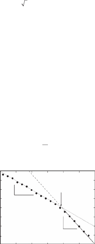
Ferrer i Cancho and Solé (2001) described a double law for Zipf; that is, the Zipan curve given by

Equation (5.16) is best described by two functions (Figure 5.6). This suggests the existence of two

regimes in English and questions the generality of Equation (5.16), as clear deviations from the expected

a ≈ 1 have been documented. This is the case for language-affecting diseases such as schizophrenia

(Ferrer i Cancho 2005a) and also certain types of words such as English nouns and verbs (Ferrer i

Cancho 2005b, 2005c). Studies on multiauthor collections of texts showed two distinct regimes for the

most frequent words (the core lexicon) and for the less frequent words (the peripheral lexicon; Ferrer

i Cancho and Solé 2001). Shakespearean works also exhibit the shape of a peripheral lexicon, which

leads to the controversial statement that it can be a case of multiauthorship (Michell 1999).

In many natural phenomena, large events are scarce but small ones quite common. For example,

there are few large earthquakes and avalanches but many small ones. There are a few words, such as

“the,” “of” and “to” that occur very frequently, but many that occur rarely, such as “Zipf.” The Zipf

law (Equation 5.16) can thus be a generalized Zipf’s law and subsequently rewritten as:

(5.17)

where the log-log plot can be linear with any slope a.

–1

–2

–3

–4

–5

–6

–7

–1.01

–1.92

Word Rank

Word Frequency

Figure 5.6 Word frequency as a function of rank for English language, showing two distinct regimes scal-

ing with a ≈ 1 (dotted line) and a ≈ 2 (dashed line). The arrow indicates the cutoff rank between the two

regimes identied as dashed and dotted lines. (Modied from Ferrer i Cancho and Solé, 2001.)

2782.indb 158 9/11/09 12:10:55 PM

Frequency Distribution Dimensions 159

This family of power laws has been successfully applied to a wide variety of problems related to

species competition (Lotka 1926) (a = 2), linguistics and social dynamics (Zipf 1949) (a = 1), and

species diversity (Frontier 1985, 1994); see also Table 5.1. In particular, Mandelbrot (1977, 1983)

demonstrates that the fractal dimensions of such power laws are given by:

= 1/a (5.18)

The original law, Equation (5.16), was further modied by Mandelbrot (1953) as:

= f

(r + f)

−a

(5.19)

Equation (5.19) has proven to be extremely useful to describe living communities in both aquatic

and terrestrial ecosystems (Frontier 1985, 1994). Thus, in Equation (5.19) f

must be thought of as

the frequency of the rth species after ranking the species in decreasing order of their frequency.

The two parameters a and f are conditioning the species diversity and the evenness of a given com-

munity, where the diversity H is given by (Shannon and Weaver 1963):

Hff

=−

∑

log

(5.20)

and the evenness J by (Pielou 1966):

log

(5.21)

where f

is the relative frequency of the species i and N is the number of species. It can be easily

seen from Equations (5.20) and (5.21) that for the same number of species, the diversity is high

when species have equivalent probability (high evenness) and low when a weak number of species

is frequent and others are scarce (low evenness). Strictly speaking, it is implicit from Equation (5.19)

that a depends on the average probability of a species; all the prerequisite conditions necessary

for the development of this species have thus been fullled. f depends on the average number of

alternatives per category of previous conditions, hence the potential diversity of the environment.

More specically, a low value of a means a slow decrease in the species abundance (that is, a more

even distribution of individuals among species), and a high value of a means a rapid decrease of

species abundance (that is, a more heterogeneous distribution). The former and the latter give less

and more vertical rank-frequency distributions (RFDs), hence high and low evenness and diversity.

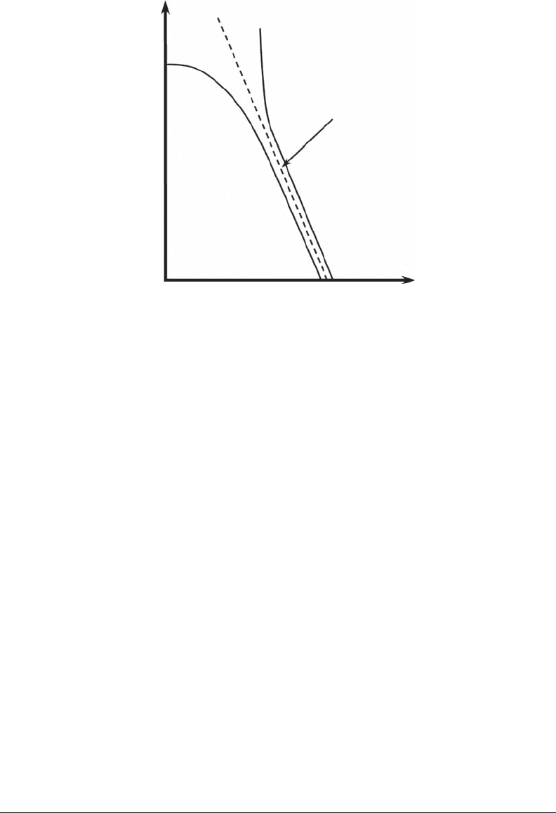
On the other hand, a positive value of f (Figure 5.7) results in a greater evenness among the most

frequent species than a higher diversity index. Alternatively, a negative f (Figure 5.7) describes a

community marked by the dominance of a few (even one) species and provides a low diversity index

and a low evenness. In summary, both f and a act upon the diversity and evenness respectively

through the niche diversity (that is, the number of alternatives in each type of previous environ-

mental condition) and through the predictability of the ecosystem (probability of the appearance

of a species when its environmental conditions are satised; Frontier 1985). Despite appealing and

meaningful properties, Equation (5.19) has seldom been used in ecology. For instance, Margalef

(1957) was the rst to t the Mandelbrot distribution to Mediterranean tintinnids with f = 0.84 and

a = 0.45, while Frontier and Bour (1976) and Frontier (1977) respectively estimated a = 1 and a =

2 for chaetognaths and pteropods. Changes in the shape of the RFDs characterize temporal changes

in the community structure (Frontier 1985). More specically, a linear-concave curve (or S-shaped

curve) indicates the dominance of one or two species that have fast growth and reproduction rates

2782.indb 159 9/11/09 12:10:57 PM

160 Fractals and Multifractals in Ecology and Aquatic Science

in a low-species-richness assemblage (that is, stage 1, pioneer community). In contrast, a more convex

shape among the rst-ranked species indicates a more even distribution among species (that is, stage

2, mature community), and a linear RFD is observed at the end of an ecological succession when the

rst-ranked species becomes more dominant and the species richness is lower (that is, stage 3, senes-

cent community). After a disturbance,* few species can quickly develop (that is, “r strategists” and

“opportunists”) so the RFD appears coarsely rectilinear with successive steps (stage 1’, intermediate

stage between stages 1 and 2) (Frontier 1985; Legendre and Legendre 2003).

5.5.4 gE n E r a l i Z E d ra n k -Fr E q u E n c y di a g r a m F o r Ec o l o g i s T s

Equations (5.16) and (5.17) can be more generally written as:

∝ r

−a

(5.22)

where X

is the value taken by any random variable relative to its rank r, and a = 1 and a ≠ 1 for the

Zipf’s and the generalized Zipf’s law, respectively. The concept related to X

is very general and refers

without distinction to frequency, length, surface, volume, mass, or concentration. Discrete processes

such as linguistics, species assemblages, and genetic structures would nevertheless still require fre-

quency computations, and thus refer to Equations (5.16) and (5.17). Alternatively, Equation (5.22) can

be thought of as a more practical alternative that can be directly applied to any continuous process.

The relevance of Equation (5.22) to describe and interpret ecological patterns is extensively discussed

and illustrated in Section 5.5.5 hereafter. Note that the appeal of both Zipf’s law (Equations 5.17, 5.19,

Here, the concept of disturbance is very general and includes, for example, seasonal overturn, massive enrichment events (such

as upwelling or eutrophication), substrate destruction (such as re or ood), and human disturbance (such as pollution).

Log f

Log r

r = 1

Log f

φ > 0

φ < 0

Figure 5.7 Schematic illustration of the expected shape of a log-log plot of the rank-frequency diagram.

The dashed line is the best t of the linear part of the rank-frequency diagram in a log-log plot, and its slope a

provides an estimate of the rank-frequency dimension as D

= 1/a. Negative and positive values of the param-

eter f lead to different shapes of the rank-frequency diagram, and describe communities marked respectively

by the dominance of a few (even one) species (low diversity and low evenness) and a greater evenness among

the most frequent species, than a higher diversity index.

2782.indb 160 9/11/09 12:11:00 PM

Frequency Distribution Dimensions 161

and 5.22) and Pareto’s law (Equation 5.11) lies in the fact that they do not require any assumptions

about the distribution of the data set or the regularity of the sampling interval, and are easy to imple-

ment. Zipf and Pareto laws have then been widely used in areas such as human demographics, linguis-

tics, genomics, and physics, but surprisingly seldom in terrestrial and marine ecology (see Table 5.1).

5.5.5 pr a c T i c a l ap p l i c a T i o n s o F ra n k -Fr E q u E n c y di a g r a m s F o r Ec o l o g i s T s

5.5.5.1 zipf’s law as a diagnostic tool to assess ecosystem complexity

Before illustrating the applicability of Zipf’s law to original data sets of centimeter-scale, two-dimen-

sional spatial distributions of bacterioplankton, phytoplankton, and microphytobenthos (Section 5.5.5.2),

the characteristic shapes expected for Zipf’s law when a distribution of interest is driven by (1) pure

randomness, (2) power-law behavior, (3) power-law behavior contaminated by internal and external

noise, and (4) competing power laws are investigated.

5.5.5.1.1 Zipf’s Law of Random Processes

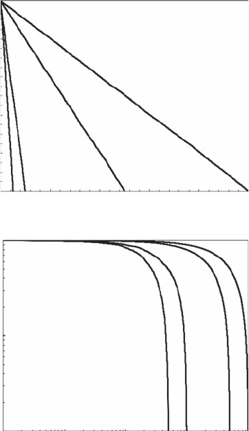
Figure 5.8 shows the characteristic signatures of ve simulated random processes (that is, white

noise) with 100, 500, 1,000, 5,000, and 10,000 data points in linear and logarithmic plots of Zipf

distributions. In linear plots (Figure 5.8A), the Zipf’s law for random noise appears as linear. On

log-log plots (Figure 5.8B), the simulated random noises do not produce any power-law behavior as

1.0

0 2,000 4,000 6,000 8,000 10,000

0.8

0.1

0.01

10 100 1,000 10,000

0.6

0.4

0.2

0.0

Figure 5.8 Linear and log-log plots of random processes with 100, 500, 1000, 50,000, and 100,000 data

points (from left to right). (Modied from Seuront and Mitchell, 2008.)

2782.indb 161 9/11/09 12:11:03 PM

162 Fractals and Multifractals in Ecology and Aquatic Science

table 5.1

nonexhaustive review of the systems studied using Pareto or zipf laws in Physical,

biological, and ecological sciences

system Pareto/zipf law reference

X-ray intensity from solar ares Pareto 1

Ecosystem model dynamics Pareto 2

Sand pile dynamics Pareto 3

Volcanic acoustic emission Pareto 4

Earthquake dynamics Pareto 5–6

Granular pile dynamics Pareto 7

Himalayan avalanches Pareto 8

Intensity of “starquakes” Pareto 9

Evolution model dynamics Pareto 10–11

Noncoding DNA sequences Zipf 12

Landscape formation Pareto 13–14

Sediment deposition in the ocean Pareto 15

Coding/noncoding DNA sequences Zipf 16

Word frequencies Zipf 17

Word frequencies Zipf 18

Formation of river networks Pareto 19–20

Rice pile dynamics Pareto 21

Noncoding DNA sequences Zipf 22

Percolation process Zipf 23

Linguistics Zipf 24

Tropical rain forest dynamics Pareto 25–27

City formation Zipf 28

Bird population dynamics Pareto 29

Aftershock series Pareto 30

City distribution Zipf 31

Discrete logistic systems Pareto 32

Procaryotic protein expression Zipf 33

Ion channels Pareto 34

Dynamics of atmospheric ows Pareto 35

U.S. rm sizes Pareto 36

Distribution of city populations Pareto 37

Economics Pareto 38

Microphytobenthos 2D distribution Pareto 39–40

Marine species diversity Zipf 41–45

Size spectra in aquatic ecology Pareto 46

Phytoplankton distribution Zipf 47–48

Sources:

McHardy and Czerny (1987);

Bak et al. (1989);

Held et al. (1990);

Diodati et al. (1991);

Feder and Feder (1991);

Olami et al. (1992);

Jaeger and Nagel (1992);

Noever (1993);

Garcia-Pelayo and Morley (1993);

Bak and

Sneppen (1993);

Paczuski et al. (1995);

Mantegna et al. (1994);

Somfai et al. (1994a);

Somfai et al. (1994b);

Rothman et al. (1994);

Mantegna et al. (1995);

Kanter and Kessler (1995);

Czirók et al. (1995);

Rigon et al.

(1994);

Rinaldo et al. (1996);

Frette et al. (1996);

Israeloff et al. (1996);

Watanabe (1996);

Perline (1996);

Solé and Manrubia (1995a);

Solé and Manrubia (1995b);

Manrubia and Solé (1996);

Makse et al. (1995);

Keitt and Marquet (1996);

Correig et al. (1997);

Marsili and Zhang (1998);

Biham et al. (1998);

Ramsden and

Vohradsky (1998);

Mercik et al. (1999);

Joshi and Selvam (1999);

Axtell (2001);

Malacarne et al. (2002);

Burda et al. (2002);

Seuront and Spilmont (2002);

Seuront and Leterme (2006);

Margalef (1957);

Frontier and

Bour (1976);

Frontier (1977);

Frontier (1985);

Frontier (1994);

Vidondo et al. (1997);

Mitchell (2004);

Mitchell and Seuront (2008).

2782.indb 162 9/11/09 12:11:04 PM

Frequency Distribution Dimensions 163

expected from Equation (5.22) but instead produce a continuous roll-off from a horizontal line (that

is, a → 0) to a vertical line (that is, a → ∞). This is representative of the fact that no value is more

likely to be more common than any other value.

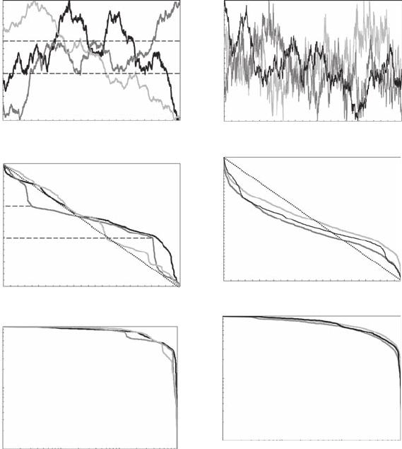
The previous observations can be extended to fractional Brownian motions (fBm) (Figure 5.9A

and Figure 5.9B). Because fBm have the desirable property of exhibiting antipersistent (an increase

in the value of the random variable is expected to be followed by a decrease) and persistent (an

increase in the value of the random variable is expected to be followed by another increase) behav-

ior, they explore a certain range of values before moving off more or less gradually to another

range of values. These properties lead to a weaker version of randomness in the Zipf framework

(Figure 5.9C,D,E,F). For antipersistent fBm (Figure 5.9A), the Zipf plots do not exhibit any clear

linear behavior (Figure 5.9C), mainly because of the upward and downward roll-off observed for

low and high rank values, respectively. This is, however, simply the result of an undersampling of

1.0AB

0.8

0.6

fBm

0.4

0.2

0.0

1.0

0.8

0.6

fBm

0.4

0.2

0.0

0 200 400

θ (Relative units)

600 800 1000 0 200 400

θ (Relative units)

600 800 1000

1.0

0.8

0.6

0.4

0.2

0.0

1.0

0.8

0.6

0.4

0.2

0.0

0.1

0.01

0.1

0.01

0 200 400

600 800 1000

0 200 400

600 800 1000

1 10

100

1000

1 10

100

1000

Figure 5.9 Antipersistent (A) and persistent (B) fractional Brownian motions (fBm), shown together with

their characteristic signatures in linear (C, D, E) and log-log (D, E, F) plots. In antipersistent and persistent

processes, an increase in the value of a random variable is expected to be followed by a decrease and an increase,

respectively. The resulting Zipf plot exhibits different deviations from randomness. The dashed lines in (B, C, D)

indicate a range of values explored by the fBM before moving off more or less gradually to another range of

values. The same colors have been used for the different fBm (A, B) and their related Zipf plots (C, D, E, F); the

darker colors characterize the more antipersistent/persistent fBm. In both cases, the symbol q represents space

or time in case of time series or transect studies, respectively. (Modied from Seuront and Mitchell, 2008.)

2782.indb 163 9/11/09 12:11:07 PM

Seuront L. Fractals and Multifractals in Ecology and Aquatic Science

Подождите немного. Документ загружается.