Seuront L. Fractals and Multifractals in Ecology and Aquatic Science
Подождите немного. Документ загружается.

164 Fractals and Multifractals in Ecology and Aquatic Science
the highest and lowest values that can be regarded as an implicit consequence of antipersistence. The
distributions are characterized by a weak evenness for high and low values, the distribution being
dominated by a few (ultimately one) high and low values. On the other hand, for persistent fBm
(Figure 5.9B), the step shape of the Zipf plot (Figure 5.9D,F) reects the property of persistent
processes to visit one particular range of values and then to change to another range sharply.
This step function becomes clearer when the fBm exhibit more persistence (Figure 5.9D,F).
The main difference between antipersistent and persistent Zipf plots then relies on the quantity
of values taken by the fBm between transitions, which will be more gradual in the antipersis-
tent case and thus contain more points than in the persistent case. Because the scale expansion
related to log-log plots may hide, at least partially, the specic structural features of Zipf plots
when compared to noise (see Figure 5.9C,D,E,F), the use of both linear and logarithmic plots is
recommended. Finally, it is stressed that any step in Zipf plots indicates structural discontinui-
ties within the data set.
3.5
3.0
2.5
2.0
X
r
= sin(3θ) +/– Noise
1.5
1.0
0.0
0.5
120
100
80
60
X
r
= (θ + 2) +/– Noise
40
20
0
120
100
80
60
X
r
40
20
0
4.0
3.5
3.0
2.5
X
r
1.5
0.5
1.0
2.0
0.0
10
1
X
r
0.1
100
10
X
r
1
02040
θ (Relative units)
A
B
CF
E
D
60 80 100 02040
θ (Relative units)
60 80 100
02040
r
60 80 100 02040
r
60 80 100
110
r
100 110
r
100
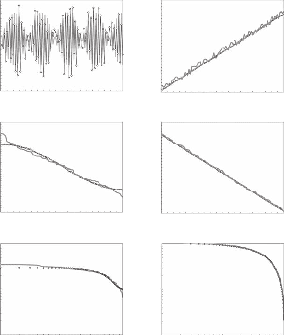
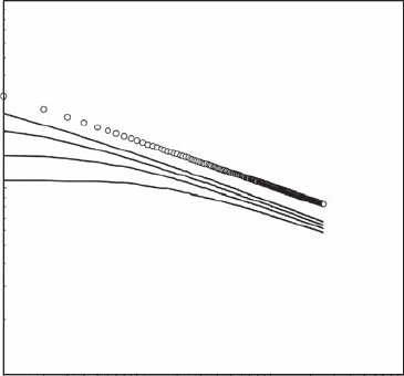
Figure 5.10 Simulated monotonic and periodic trends before (gray curve) and after (open diamonds) being
contaminated by observational white noise (A, D), their subsequent Zipf signatures in linear (B, C), and log-
log (D, E) plots. In both cases, the symbol q represents space or time in case of time series or transect studies,
respectively. (Modied from Seuront and Mitchell, 2008.)
2782.indb 164 9/11/09 12:11:09 PM
Frequency Distribution Dimensions 165
5.5.5.1.2 Zipf’s Law of Deterministic Processes
Deterministic patterns and processes are well known in time-series analysis and referred to as
monotonic and periodic trends. Gradients and sine waves are archetypical examples. Periodicity
is common in both terrestrial and marine ecology. Here, we simulate an increasing linear trend
and a sine wave trend. Both of them have been subsequently contaminated by observational white
noise (Figure 5.10A,D). The Zipf plots of the increasing trends exhibit the characteristic signature
of white noise (Figure 5.10B,C). In contrast, the Zipf plots of the sine waves exhibit distinct features
(Figure 5.10E,F). The sine wave has the characteristic Zipf shape of a pattern oversampled for its
higher and lower values, while the noisy sine wave converges toward a random Zipf signature.
5.5.5.1.3 Zipf’s Law of Pure Power Laws
Patterns and processes characterized by a power law function (for example, Equation 5.22) will
appear as a straight line in log-log plots (Figure 5.11). However, this theoretical case is rare in
nature, and a more realistic series where power laws may be hidden by a wide range of contaminat-
ing processes is investigated hereafter.
5.5.5.1.4 Zipf’s Law of Contaminated Power Laws
Before focusing on the processes susceptible to modify the characteristic exponents of Zipf power laws,
we will consider the potential effects of external and internal noise on the extent of the power laws. In
the rst approach, the variability of a given descriptor is driven by “new” events, which represent exog-
enous variables (exogenous in the sense that they are not a part of an internal mechanism that drives
the descriptor uctuations), for instance, the motion of dinoagellate cells induced by vertical turbulent
eddy diffusivity. On the other hand, internal noise refers to the existence of an engine within the cells
(that is, endogenous) that generates motion by mechanisms of feedback of the motion of the cells upon
themselves.
5.5.5.1.4.1 Zipf’s Law of Power Laws Contaminated by External (White) Noise
If varying amounts of noise are added to the power function X
r
∝ r
−a
as:
Y
r
= (r
−a
+ e) (5.23)
1
0.1
0.01
0.001
0.0001
0.00001
100010010
r
Y
r
1
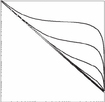
Figure 5.11 Log-log signature of a power law (dots) with different percentage of additive noise (0.01%,
0.1%, 1%, and 10%, from bottom to top). (Modied from Seuront and Mitchell, 2008.)
2782.indb 165 9/11/09 12:11:12 PM
166 Fractals and Multifractals in Ecology and Aquatic Science
where e is a white noise whose amplitude is dened as being a given percentage of the maximum
value of X
r
, then the noise causes a rightward departure from the straight line at a rank proportional
to the amount of noise added (Figure 5.11). Measuring the point of departure from a power law for
a variety of noise levels (here, 0.01%, 0.1%, 1%, and 10%) recovers the original function for Zipf
plots. Such a graphical approach could be very valuable to estimate the extent to which noise con-
taminates or contributes to the measured signal.
Consider two situations where a simulated power-law function (X
r
∝ r
−a
, with a = 0.18) is mixed with
a random noise e
1
, vertically offset so as not to overlap, that is, e
2
∈ [min X
r
, c
1
] and e
2
∈ [c
2
, min X
r
], as
50
40
30
Y
r
= (X
r
+ ε
1
)
20
0
10
50
40
30
Y
r
= (X
r
+ ε
2
)
20
0
10
50
40
30
Y
r
= (X
r
+ ε
1
)
20
0
10
050
A
B
C
100 150 200 250
θ (Relative units)
300 350 400 450
050 100 150 200 250
θ (Relative units)
300 350 400 450
050 100 150 200 250
θ (Relative units)
300 350 400 450
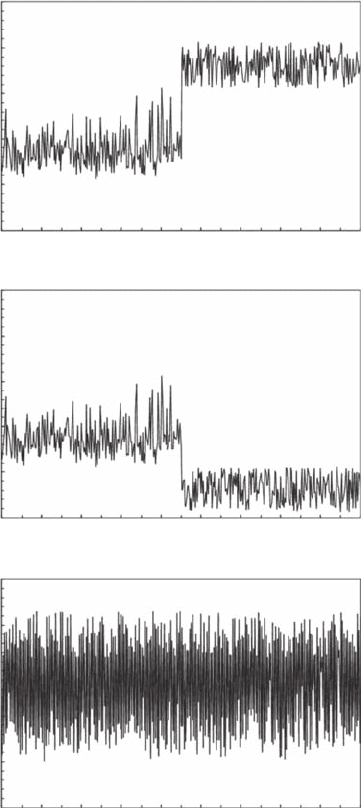
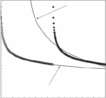
Figure 5.12 Power-law distribution X
r
∝ r
−
0.18
combined with a white noise distribution e
i
as Y
r
= X
r
+ e
i
,
as a caricature of two populations separated by a sharp gradient (A, B), or mixed (C). The two populations,
characterized by a power law X
r
and a random distribution e
i
, have been considered as fully separated (A, B),
with e
i
= e
1
(e
1
∈ [max X
r
, c
1
]) and e
i
= e
2
(e
2
∈ [c
2
,
max X
r
]), and fully mixed, with e
i
= e
1
(C). The symbol q
represents space or time in case of time series or transect studies, respectively. (Modied from Seuront and
Mitchell, 2008.)
2782.indb 166 9/11/09 12:11:14 PM
Frequency Distribution Dimensions 167
Y
r
= X
r
+ e
i
. This could illustrate the expected outcome of a transect crossing a boundary separating
two distinct structural entities or a vertical prole crossing a strong thermocline (Figure 5.12A,B).
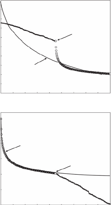
In both cases, the subsequent Zipf plots exhibit a clear step function indicative of a structural dis-
continuity (Figure 5.13A,B) between the characteristic behaviors expected in cases of randomness
and power law. However, while we used the same power law in both cases, the exponents and the
goodness of the power-law ts are different (Figure 5.13).
This result could lead to misinterpretation of Zipf plots. The widely acknowledged assump-
tion that any range of values with the same extent (for example 10 to 100, or 10,000 to 10,090)
on the x axis produces the same range of values of the y axis is no longer valid in the nonlinear
framework of power laws. Thus, different ranges of rank, r, values 225 to 450 (Figure 5.12A)
and 1 to 450 (Figure 5.12B), return different ranges on the y axis, and thus different laws. As
a consequence, to conduct Zipf analyses successfully and for the results to be meaningful, we
recommend separate analyses of the different ranges of values identied in a preliminary global
analysis as being separated by a step function. Figure 5.14 thus illustrates how the simulated
50
40
30
Y
r
= (X
r
+ ε
1
)
20
10
Y
r
= 16.9r
–0.83
Y
r
= 27.98r
–0.18
0
30
Y
r
= (X
r
+ ε
2
)
20
10
0
0 150
A
B
300
r
450
0 150 300
r
450
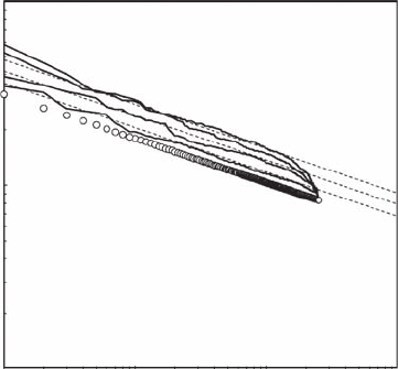
Figure 5.13 Zipf plots of the two theoretical situations illustrated in Figure 5.12A (A) and Figure 5.12B (B).
Note that while the same power laws have been used in both situations, the original power law X
r
∝ r
−
0.18
is
recovered only when X
r
> e
i
(b); when X
r
< e
i
the power law t to the power law population is not signicant (A).
The circles indicate the step function behavior of the Zipf plot that should be regarded as being indicative of
structural changes within the data set. (Modied from Seuront and Mitchell, 2008.)
2782.indb 167 9/11/09 12:11:17 PM
168 Fractals and Multifractals in Ecology and Aquatic Science
power law X
r
∝ r
−a
is recovered by separately analyzing the values characterized by ranks rang-
ing from 225 to 450 for e
1
(see Figure 5.12A and Figure 5.13A).
The combination of randomized values of the power law X
r
∝ r
−a
and the nonoverlapping noise,
e
i
, (Figure 5.12A,B,C), leads to results similar to those in Figure 5.13. Zipf analysis is then revealed
to be extremely powerful and valuable in the identication and quantication of hidden structural
properties of any data sets.
5.5.5.1.4.2 Zipf’s Law of Power Laws Contaminated by Internal (Process) Noise
Instead of considering an external process (that is, observational or instrumental noise), the power law
itself can be contaminated by internal variability. In such cases, the power-law function X
r
∝ r
−a
(with
a = 0.18) is rewritten as
Y
r
= (r ± r × e)
−a
(5.24)
where e is still a white-noise term whose amplitude is dened as being a given percentage of the
maximum value of X
r
, here randomly chosen as being positive or negative. Whatever the amount
of noise considered (here, between 5% and 100%), the exponents a estimated from Equation (5.24)
cannot be statistically regarded as being different from the expected values of 0.18 (p < 0.01).
5.5.5.1.5 Zipf’s Law of Competing Power Laws
5.5.5.1.5.1 Case Study 1: Mixing Noninteracting Species
Consider two theoretical phytoplankton populations separated by a sharp hydrological gradient.
One is composed of diatoms that can reasonably be thought of as following a power-law form,
X
r
∝ r
−a
(here, a = 0.18), with respect to their large size and aggregative properties. The other one
is composed of dinoagellates that, because of their smaller size, high concentration, and motility
are more homogeneously distributed and are then simply represented here as a background con-
centration k
i
. The resulting pattern can then be thought of as the combination Y
r
= X
r
+ k
i
. It is
emphasized here that any change in the background concentration k
i
does not affect the power-law
nature of the original data set X
r
. However, the exponent a′ of the resulting power laws Y
r
∝ r
−a
′
decreases with increasing values of k
i
. The addition of an increasing background concentration
30
25
20
15
10
5
0
050 100 150 200
r
250
Y
r
= 27.98r
–0.18
Y
r
= 1395r
–0.81
300 350 400 450
Y
r
= (X
r
+ ε
1
)
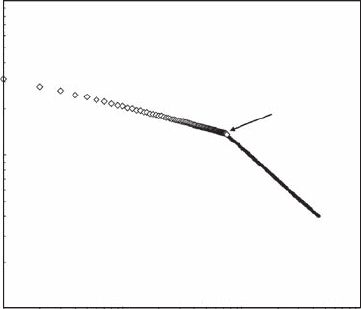
Figure 5.14 Density dependence of a Zipf plot. The Zipf behavior of the power-law population X
r
character-
ized by X
r
> e
i
(black squares) (Figure 5.13A), is recovered (open squares) when the range of values identied
as being separated by a step function (see Figure 5.13A,B) have been analyzed separately. (Modied from
Seuront and Mitchell, 2008.)
2782.indb 168 9/11/09 12:11:22 PM
Frequency Distribution Dimensions 169
thus smoothed out the differences between ranks. The observation of such a decrease in empirical
power-law exponents from eld data sampled at the same point before and after the disruption of a
hydrological gradient, or at different period of the seasonal cycle, would strongly indicate a struc-
tural change in the relative organization of the studied biological communities.
Now consider a situation where two spatially separated phytoplankton populations are mixed—
for example, two monospecic diatom populations—characterized by overlapping ranges of con-
centrations and distinct power-law forms, X
1r
∈ [2.99, 13.79] and X
1r
∝ r
−a
1
with a
1
= 0.18, and X
2r
∈
[3.19, 31.37] and X
2r
∝ r
−a
2
with a
1
= 0.24, respectively. Evenly mixing these two populations with-
out considering any interactions will result in the Zipf structures shown in Figure 5.15. The range of
values corresponding to the overlapping of the two power laws presents an intermediate power-law
behavior with a characteristic exponent a′ = 0.196 (Figure 5.15). More generally, the values of a′
are implicitly bounded between a
1
< a′ < a
2
, where a
1
and a
2
are the Zipf exponents of the original
power laws and depend on the proportion of values from each original power law, following a′ =
ka
1
+ (1 − k)a
2
. Finally, as stated above, a separate analysis of the values greater than the critical
concentration (13.79) associated with the step function shown in Figure 5.15 is necessary to recover
the original exponents a
2
= 0.24.
5.5.5.1.5.2 Case Study 2: Mixing Interacting Species
Here, we consider one of the previous phytoplankton populations whose concentration X
r
is charac-
terized by a power-law form X
r
∝ r
−a
, with a = 0.24. We will now investigate the effects of processes
capable of locally decreasing (that is, mortality related to inter- and intraspecic competition, or
grazing) or increasing (phytoplankton growth or coagulation processes) phytoplankton concentra-
tion on the Zipf signature of the population X
r
∝ r
−0.24
. Note that while the following examples are
based on the interactions between phytoplankton and zooplankton organisms, this does not hamper
the generality of the results, as the same approach can be used to describe the interactions between
terrestrial plants and grazers.
Decrease in local phytoplankton concentration. First, under the assumption of evenly distrib-
uted grazers, the grazing impact of copepods can be estimated as a percentage or a Michaelis-
Menten function of the local phytoplankton concentration. Assuming the ingestion of phytoplankton
cells by copepods is a percentage of a random function of food availability, the resulting food
100
10
1
1 10010 1000
r
Y
r
Figure 5.15 Log-log plot signature of the Zipf behavior resulting from mixing two theoretical populations
characterized by two distinct power laws and overlapping ranges of concentrations. The range of values corre-
sponding to the overlapping of the two power laws presents an intermediate power-law behavior with a character-
istic exponent a′ dened as a
1
< a′ < a
2
and a′ = ka
1
+ (1 − k)a
2
. (Modied from Seuront and Mitchell, 2008.)
2782.indb 169 9/11/09 12:11:25 PM
170 Fractals and Multifractals in Ecology and Aquatic Science
distributions can be described by
Y
1r
= X
r
− kX
r
(5.25)
and
Y
2r
= X
r
− eX
r
(5.26)
where k is a constant, 0 ≤ k ≤ 1, and e is a random-noise process, that is, e ∈ [0, 1]. For increasing
values of k, the function Y
1r
is simply shifted downward on a log-log Zipf plot (not shown), indicat-
ing a decrease in the background concentration of the population. A similar trend can be identied
in the variable Y
2r
for an increasing amount of noise, but with a characteristic “noise roll-off” for
low rank values (Figure 5.16).
Alternatively, following laboratory data on the feeding of copepods suggesting that ingestion
rate can be fairly represented by a Michaelis-Menten function (see, for example, Mullin et al. 1975),
Equations (5.25) and (5.26) are modied as:
Y
3r
= X
r
− I
max
X
r
/(k
s
− X
r
) (5.27)
where I
max
is the maximum ingestion rate, k
s
is the half-saturation constant for feeding, and X
r
the
concentration of food. Figure 5.17 shows the Zipf structure of the resulting phytoplankton concen-
tration Y
3r
for different values of the half-saturation constant k
s
and the maximum ingestion rate I
max
.
It clearly appears that the effect of grazing is mainly perceptible for low values of Y
3r
, a direct conse-
quence of the convex form of the Michaelis-Menten function (see Equation 5.27), and leads to a sig-
nicant divergence from a power law when I
max
is high and k
s
is low (compare Figure 5.17A,B,C).
However, the two previous approaches are implicitly based on the hypothesis of a homogeneous
phytoplankton distribution, which is now recognized as an oversimplied hypothesis (Seuront et al.
1996a, 1999; Waters and Mitchell 2002; Waters et al. 2003) and did not take into account potential
behavior adaptation of grazers to varying food concentrations (Tiselius 1992). If one considers
that the remote sensing abilities (Doall et al. 1998) of copepods can lead to aggregation of grazers
in areas of high phytoplankton concentrations as investigated both empirically and numerically
(Tiselius 1992; Saiz et al. 1993; Leising and Franks 2000; Seuront et al. 2001), Equation (5.26) can
be modied as:
Y
4r
= X
r
− 10
(X
r
/k)
(5.28)
100
10
1
1 10010 1000
r
Y
2r
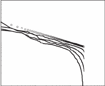
Figure 5.16 Log-log plot signature of the Zipf behavior expected in case of a power law X
r
(open dots) com-
peting with a random mortality component (Y
2r
= X
r
− eX
r
), e = 0.05, 0.25, 0.50, and 0.75 (from top to bottom).
(Modied from Seuront and Mitchell, 2008.)
2782.indb 170 9/11/09 12:11:28 PM
Frequency Distribution Dimensions 171
100
10
0.1
1
1
I
max
= 30
I
max
= 20
I
max
= 10
10010 1000
r
Y
3r
100
10
1
1 10010 1000
r
Y
3r
100
10
1
1 10010 1000
r
Y
3r
A
B
C
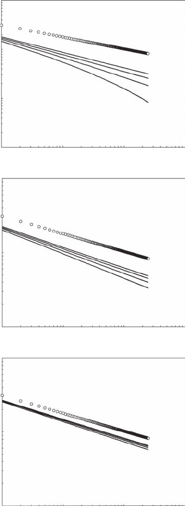
Figure 5.17 Log-log plot signature of the Zipf behavior expected in case of a power law X
r
(open dots) com-
peting with a Michaelis-Menten grazing component (Y
3r
= X
r
− I
max
X
r
/(k
s
+ X
r
)). For a given maximum ingestion
rate I
max
, the effect is stronger for high values of the half-saturation constant k
s
. (Modied from Seuront and
Mitchell, 2008.)
2782.indb 171 9/11/09 12:11:30 PM
172 Fractals and Multifractals in Ecology and Aquatic Science
where k is a constant and the ingestion function I(X
r
) = 10
(X
r
/k)
represents an increased preda-
tion impact on higher phytoplankton concentration. The advantage of the function I(X
r
) is that
it can be regarded as a representation of both aggregation of copepods with constant ingestion
rates and evenly distributed copepods with increasing ingestion rates in high-density phytoplankton
patches. Decreasing values of the constant k increases the grazing impact on high-density patches
(Equation 5.28). The grazed phytoplankton population then diverges from a power-law form for
high values of Y
4r
but asymptotically converges to the original power law for the smallest values
of Y
4r
; that is, Y
4r
∝ r
−a
for r → r
min
(Figure 5.18).
Although the previous examples are based on zooplankton grazing on phytoplankton, we never-
theless stress the generality of our approach, as similar results could have been obtained considering
two phytoplankton populations competing for the same nutrient resource using Michaelis-Menten
or Droop functions.
Increase in local phytoplankton concentration. For the sake of simplicity, consider that phyto-
plankton growth (in response to physical coagulation or nutrient uptake) could be represented as a
percentage or a random function of the actual phytoplankton concentration X
r
. Equations (5.25) and
(5.26) are then respectively rewritten as:
Y
5r
= X
r
+ kX
r
(5.29)
and
Y
6r
= X
r
+ eX
r
(5.30)
where k is a constant, 0 ≤ k ≤ 1, and e is a random noise process, that is, e ∈ [0, 1]. For increasing
values of k, the function Y
5r
is, in full agreement with what has been concluded from Equation
(5.25), shifted upward on a log-log Zipf plot (not shown), indicating an increase in the background
concentration of the population. Using different values of k in Equation (5.29) has no effect on the
shape of the related Zipf plots and exponents a′ (Y
5r
∝ r
−a
′), which remain equal to the original
100
10
1
1 10010 1000
r
Y
4r
Figure 5.18 Log-log plot signature of the Zipf behavior expected in case of a power law X
r
(open dots) com-
peting with a preferential grazing component for high phytoplankton concentrations (Y
4r
= X
r
− 10(X
r
/ k
s
)). The
grazed phytoplankton population diverges from a power-law form for high concentrations, but asymptotically
converges to the original power law for the smallest values. The extent of the observed divergence is controlled
by increasing grazing pressure k (from top to bottom). (Modied from Seuront and Mitchell, 2008.)
2782.indb 172 9/11/09 12:11:32 PM
Frequency Distribution Dimensions 173
power law, that is, Y
5r
∝ r
−0.24
. Slightly different conclusions can be drawn from the behavior of
the Zipf plots of function Y
6r
(Figure 5.19). First, increases in the amount of noise e (ranging from
25% to 100%) lead to a vertical offset of function Y
6r
when compared to the original power law.
The resulting functions exhibit the characteristic downward roll-off signature related to random-
ness and might also locally show increasing trends that are intrinsically caused by the random
component in Equation (5.30). They could be misleading, especially when they occur over the
highest rank range and must not be related to breakpoints indicative of structural discontinuities
that would erroneously lead to a separate analysis of different subsections of the original data set.
Finally, even if the exponents a′ uctuate around the original value, they are never signicantly
different (p < 0.05).
Increase vs. decrease in local phytoplankton concentration. Because the two previous situations
are unlikely to be found individually in the ocean but should also occur concomitantly, combining
Equations (5.25) and (5.29) with Equations (5.26) and (5.30) leads to:
Y
7r
= X
r
+ (k
1
− k
2
) X
r
(5.31)
and
Y
8r
= X
r
+ (e
1
− e
2
) X
r
(5.32)
where k
1
and k
2
are constants (0 ≤ k
1
≤ 1, and 0 ≤ k
2
≤ 1), and e
1
and e
2
are random-noise processes;
that is, e
1
∈ [0, 1] and e
2
∈ [0, 1]. The resulting functions Y
5r
and Y
6r
exhibit intermediate behaviors
between what have been observed from Equations (5.25) and (5.29), and Equations (5.26) and (5.30).
For k
1
= k
2
, the original power law, Y
7r
∝ r
−0.24
, is recovered; the growth component compensates
for the death component. In contrast, when k
1
< k
2
and k
1
> k
2
, the resulting function Y
7r
is shifted
downward and upward on a log-log plot as previously observed from Equations (5.25) and (5.29).
Although the overall structure is preserved, the latter and the former cases lead to decreases and
increases in the background concentration of the population. The Zipf plot of function Y
8r
, shown in
100
10
1
1 10010 1000
r
Y
6r
Figure 5.19 Log-log plot signature of the Zipf behavior expected in case of a power law X
r
(open dots) com-
peting with a random growth component (Y
6r
= X
r
− eX
r
), where e = 0.25, 0.50, 0.75, and 1.00 (from bottom to
top). The arrows indicate the minimum of a range of Y
6r
values locally diverging from a power law because of
successively increasing random increments. The dashed lines indicate slope of the power-law behavior of the
initial values X
r
. (Modied from Seuront and Mitchell, 2008.)
2782.indb 173 9/11/09 12:11:35 PM