Russ J.C. Image Analysis of Food Microstructure

Подождите немного. Документ загружается.

For some purposes, such as locating spots on electrophoresis gels, the absolute

coordinates are important (in that case, the density-weighted centroid seems the

most reasonable choice). In many more applications, it is neighbor distances that

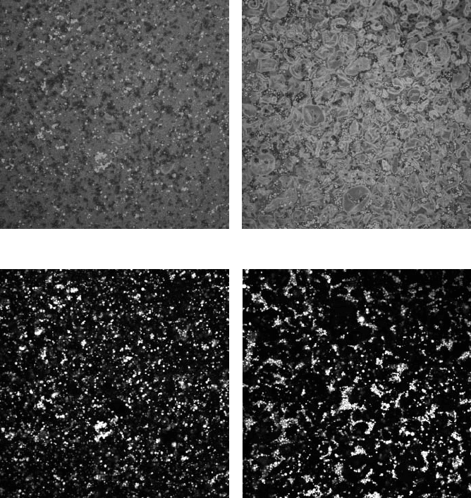
provide a way to measure spatial distributions. In the example shown in Figure 5.29,

the two different custards have visually obvious differences in the uniformity with

which the fat globules are dispersed. They have been processed by thresholding the

red channel in a color image (because they were stained with Nile Red) and plotting

the ultimate eroded points (the local peaks in the Euclidean distance map), which

were then used as the locations of the features.

(a) (b)

FIGURE 5.29 Measuring the spatial dispersion of fat in custard (courtesy of Anke M. Jan-

ssen, ATO B.V., Food Structure and Technology): (a, b) two custards (see Color Figures 3.56

and 4.7; see color insert following page 150); (c, d) thresholded red channels.

2241_C05.fm Page 317 Thursday, April 28, 2005 10:30 AM

The nearest neighbor distances are calculated with the Pythagorean theorem

from the absolute coordinates of the features in the image. A search is needed to

locate the minimum value, but with modern computers this is very fast for images

containing only hundreds or thousands of features. The key to using nearest neighbor

distance as a measure of spatial distribution lies in the characteristics of a random

distribution, in which each feature is independent and feels no force attraction or

repulsion from the others (like sprinkling pepper onto a table). In that case, as shown

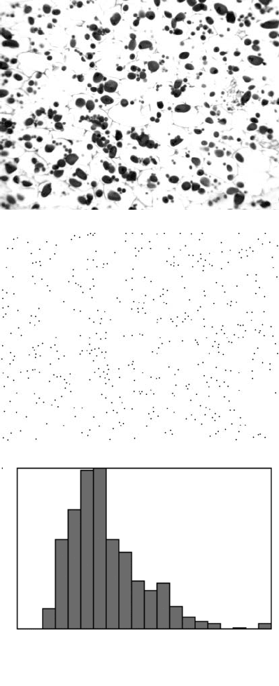
in Figure 5.30, the nearest neighbor distances have a Poisson distribution. This is

the hallmark of a random distribution. The Poisson distribution has very simple

statistical properties, one of which is that the mean value can be calculated simply

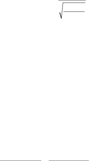
from the number of points. For a random distribution the mean nearest neighbor

distance will be

(5.3)

For the starch granules in potato tissue shown in Figure 5.30 the histogram has

the shape of a Poisson distribution and a mean value of 35.085 (pixels). The calcu-

lated mean nearest neighbor distance for 447 features in an image that is 1600 ×

1200 pixels in size is 32.76. These values are statistically indistinguishable for that

number of features so we would conclude that the distribution of starch grains cannot

be distinguished from random.

If the features are clustered together, the mean nearest neighbor distance is less

than that calculated using the equation for the random distribution. Conversely if

they are self-avoiding, the actual mean nearest neighbor distance is greater. The ratio

of the actual mean nearest neighbor distance to the value calculated for a random

spatial distribution is a useful measure of the tendency of the distribution toward

clustering or self-avoidance. Since the distance values are compared only as ratios,

the actual image calibrated magniﬁcation is not needed for this purpose.

Applying this procedure to the fat globules in the images of Figure 5.29 reports

the following results:

From these results it is evident that one of the two custards has a random distribution

of fat globules, but in the other there is clustering present.

Conversely, Figure 4.41 of Chapter 4 showed a distribution of protein bodies

and starch granules that were self-avoiding. There can be many reasons for clustering

Actual Mean Calculated Mean

Image

Nearest Neighbor

Distance (in.)

Distance for

Random case (in.)

Figure 25(c)0.12880.0985

Figure 25(d)0.12540.1248

Mean Nearest Neighbor Distance =

Number

Area

0.5

2241_C05.fm Page 318 Thursday, April 28, 2005 10:30 AM

(a)

(b)

(c)

FIGURE 5.30 The spatial distribution of starch granules in potato: (a) magenta channel from

the color image in Chapter 3, Figure 3.57 and Color Figure 3.57 (see color insert folllowing

page 150); (b) ultimate eroded points for the starch granules; (c) distribution plot of measured

nearest neighbor distances.

Min = 0 Nearest Neighbor Distance(µm) Max = 100

To tal = 447, 20 bins

Mean = 35.0851, Std. Dev. = 15.5192

Skew = 1.62929, Kurtosis = 8.47838

Count

2241_C05.fm Page 319 Thursday, April 28, 2005 10:30 AM

or self-avoidance, including chemical depletion, surface tension, electrostatic forces,

etc. Finding that a non-random structure is present is only the ﬁrst step in under-

standing the reasons for the structure to have formed. Figure 5.14 showed an image

of rice grains dispersed for length measurement. The means of dispersal, a vibrating

table, should produce mechanical interactions between the grains causing them to

separate. Measuring the mean nearest neighbor distance produces a result of 5.204 mm,

which is much greater than the value of 2.440 mm predicted for a random distribu-

tion. This conﬁrms the (expected) self-avoiding nature of the dispersal.

In this image there is a signiﬁcant difference between the nearest neighbor

distance based on centroid-to-centroid spacing and the distance of closest approach

or minimum separation between features. Figure 5.31 shows plots of the two different

distances, and Figure 5.32 illustrates the meaning of the two parameters. In many

structures, the identity of the feature that is nearest by one deﬁnition is not even the

same as that which is closest by the other, which leads to some interesting but

complex possibilities for performing statistical analysis on neighbor pairs. It is also

interesting to observe that the nearest neighbor directions and the feature orientations

in the rice image are not isotropic, as shown in Figure 5.33. In other words, there

(a)

(b)

FIGURE 5.31 Plots of the distribution of nearest neighbor distance for the rice grains in

Figure 5.14: (a) based on centroid-to-centroid distance; (b) based on the minimum edge-to-

edge separation distance.

3.054

Nearest Neighbor Distance (mm)

8.409

Count

Total = 261

0.0

Minimum Separation Distance (mm)

3.0

Count

Total = 261

2241_C05.fm Page 320 Thursday, April 28, 2005 10:30 AM

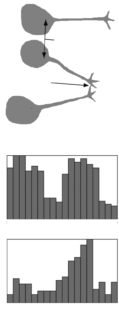
FIGURE 5.32 Diagram illustrating the nearest neighbor distance based on centroid-to-cen-

troid spacing and edge-to-edge minimum separation, which may not be to the same neighbor.

(a)

(b)

FIGURE 5.33 Plots revealing anisotropy in the rice grains in Figure 5.14: (a) nearest neighbor

direction; (b) orientation angle of the grains.

Nearest

Neighbor

Distance

Minimum

Separation

Distance

Nearest Neighbor Direction (deg)

360

Count

Total = 261

Orientation Angle (deg)

180

Count

2241_C05.fm Page 321 Thursday, April 28, 2005 10:30 AM

is a tendency toward alignment of the features, as might be expected from consid-

eration of how the dispersal is accomplished.

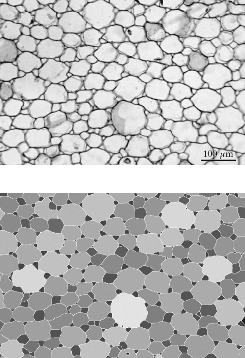
Another type of neighbor relationship is the number of adjacent features, which

is often the same as the number of sides on a polygonal feature. This arises most

often in cell structures such as the corn plant section in Figure 5.34. In three

dimensions the cells are polyhedra. Where the section plane cuts through the center

of a cell, it produces a polygon with many sides and a large number of adjacent

(a)

(b)

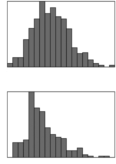
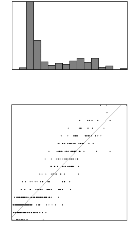
FIGURE 5.34 Section through corn plant tissue: (a) original image; (b) cells with grey scale

values representing the number of touching neighbors; (c) plot of the number of sides (note

the large number of three-sided cell sections); (d) regression plot of number of adjacent

neighbors vs. cell size.

2241_C05.fm Page 322 Thursday, April 28, 2005 10:30 AM

neighbors. While the number of neighbors seen in the section is less than the number

of touching neighbors in three dimensions, the analysis of number of neighbors still

reveals some important characteristics of different types of structures. The maximum

shown in the image is a cell with 16 neighbors. Where the location of the cut passes

through a corner of the three-dimensional cell it produces a small section with a

small number of sides. Note the very large number of three-sided sections, most of

which occupy positions between the larger cells. As shown in the ﬁgure, there is a

strong correlation between size and number of adjacent neighbors.

(c)

(d)

FIGURE 5.34 (continued)

223

Count

Min = 1 Adjacent Feature Count Max = 16

Mean = 4.42485, Std. Dev.=4.27309

To t al = 717

Adjacent Feature Count

min=1.128 Equivalent Circular Diameter

max=124.7

Equation: Y = 0.12385 * X + 1.25098

R-squared = 0.91532, 517 points

2241_C05.fm Page 323 Thursday, April 28, 2005 10:30 AM

GRADIENTS

One major reason for interest in the location of features is to discover and

characterize gradients in structure. Most natural materials, and many manufactured

ones, are far from uniform, but instead have systematic and consistent variations in

size, shape, density, etc., as a function of location. In many cases, the direction of

the gradient is perpendicular to some surface or boundary. The complexity of struc-

ture and the natural variation in the size, shape, density, etc. of the individual features,

can make it very difﬁcult to detect visually the true nature of the gradient. Hence,

computer measurement may be required.

Depending on the image magniﬁcation and the scale of the gradient, position

may be measured by the Euclidean distance map or by simple X- or Y-coordinates.

If the distance from some boundary or feature within the image is important, the

EDM is the tool of choice. This was illustrated in Figures 4.42 to 4.44 in Chapter

4. For situations such as determining a gradient normal to a surface, if the image

shows a section taken perpendicular to the surface, the Y-coordinate of a feature in

the image may provide the required position information. In either case, plots of

feature property vs. position are used to reveal and characterize the gradient.

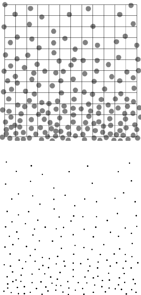
As an example, Figure 5.35 repeats a diagram from Chapter 1 (Figure 1.13).

Instead of counting the number of hits made by points in a grid to estimate the vertical

gradient, as done there, procedures based on feature measurement will be used. A

plot of area fraction vs. vertical position can be generated by counting the number

of pixels covered by features at each vertical position (Figure 5.35c). However, that

is not a feature-speciﬁc measurement. Visually, the nearest neighbor distance for

each feature changes most strikingly from bottom to top of the image. Reducing

each feature to its ultimate eroded point and measuring the nearest neighbor distance

for each feature produces a graph (Figure 5.35d) that shows this gradient.

All of the features in the preceding example were identical in size and shape, it

is only their distance from their neighbors that varies. More often the variation is

in the size, shape and density parameters of the individual features. In the example

in Figure 5.36, the size of each cell in plant tissue is measured. The procedure used

was to threshold the image, skeletonize the binary result and then convert the skeleton

to a 4-connected line that separates the cells. Measurement of the size (equivalent

circular diameter) of each cell and plotting it against the horizontal position (of the

centroid) produces the result shown in Figure 5.36(e). This plot is difﬁcult to

interpret, because of the scatter in the data. The band of small cells about 40% of

the way across the width of the image is present, but not easy to describe. Interpre-

tation of the data can be simpliﬁed by coloring each cell with a grey scale value

that is set proportional to the size value (Figure 5.36d). A plot of the average pixel

brightness value as a function of horizontal position averages all of the size infor-

mation and shows the location of the band of small cells, as well as the overall

complex trend of size with position.

Sometimes the color coding of features is not even required. In the example of

Figure 5.37, an intensity plot on the original image sufﬁces to show the structural

gradient. The image is a cross-section of a bean. There is a radial variation in cell

2241_C05.fm Page 324 Thursday, April 28, 2005 10:30 AM

(a)

(b)

FIGURE 5.35 Measuring a vertical gradient: (a) original with superimposed grid; (b) ultimate

eroded points; (c) plot of area fraction vs. position; (d) plot of nearest neighbor distance vs.

position.

2241_C05.fm Page 325 Thursday, April 28, 2005 10:30 AM

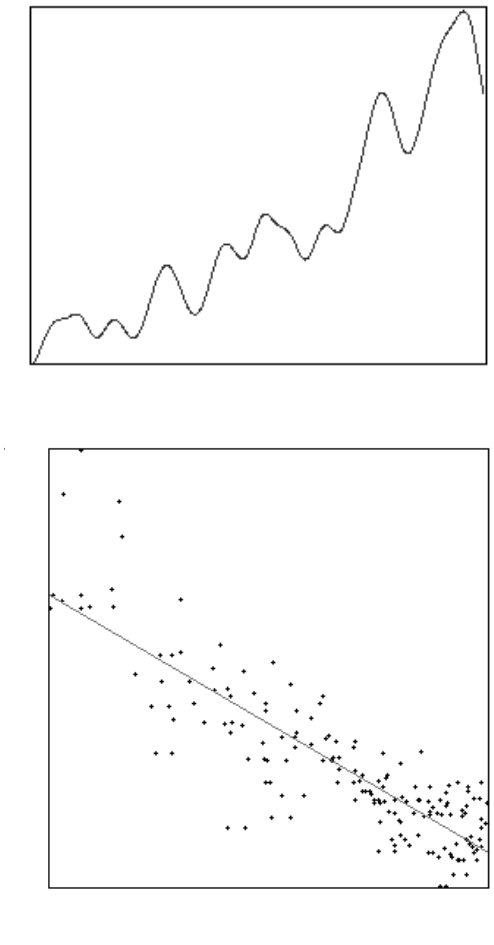
(c)

(d)

FIGURE 5.35 (continued)

Ver tical Position

Area Fraction (%)

72.12

13.41

Nearest Neighbor Distance

min=15 Vertical Position (pixels) max=507

Equation: Y = -0.07013 * X + 53.7397

R-s

uared = 0.86095

168

oints

2241_C05.fm Page 326 Thursday, April 28, 2005 10:30 AM