Russ J.C. Image Analysis of Food Microstructure

Подождите немного. Документ загружается.

SIZE DISTRIBUTIONS

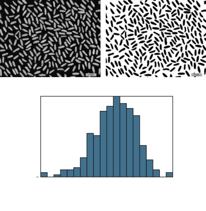
Distributions of the sizes for natural objects such as rice grains often produce

normal distributions. Statisticians know that the central limit theorem predicts that

in any population for which there are a great many independent variables (genetics,

nutrients, etc.) that affect a property such as size, the result tends toward a normal

distribution. The statistical interpretation of data is somewhat beyond the intended

scope of this text, but statistical properties such as the skew (ideally equal to 0) and

kurtosis (ideally equal to 3) are often used to judge whether a distribution can be

distinguished from a Gaussian, and a chi-squared test may also be used.

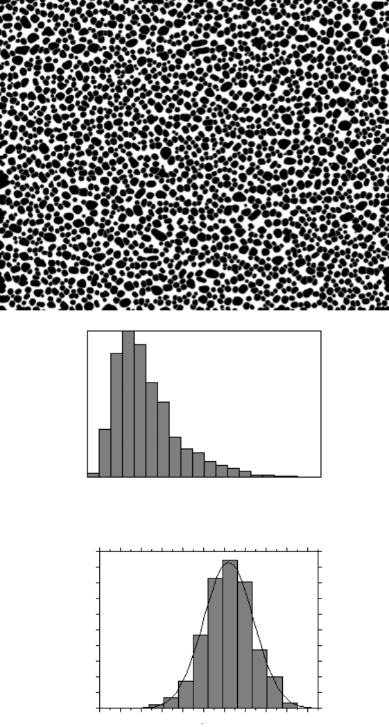
Another common type of distribution that arises from many thermodynamic

processes is a log-normal curve, with a few large features and many small ones. The

ice crystals in ice cream shown in Figure 5.15 provide an example. The sizes (areas

(a) (b)

(c)

FIGURE 5.14

Measurement of the length of rice grains: (a) original image; (b) thresholded;

Min = 0.56

Max = 0.95

Total = 261, 20 bins

Mean = 0.78088, Std.Dev.=0.06404

Skew = -0.40239, Kurtosis = 3.45471

Count

Length (cm)

2241_C05.fm Page 297 Thursday, April 28, 2005 10:30 AM

(a)

(b)

FIGURE 5.15

Ice crystals in ice cream (after some remelting has caused rounding of cor-

ners); (a) original image, courtesy of Ken Baker, Ken Baker Associates); (b) thresholding the

feature outlines; (c) ﬁlling the interiors and performing a watershed segmentation; (d) distri-

bution of sizes (area, with measurements in pixels); (e) replotted on a log scale with a

superimposed best-ﬁt Gaussian curve for comparison.

2241_C05.fm Page 298 Thursday, April 28, 2005 10:30 AM

(c)

(d)

(e)

FIGURE 5.15 (continued)

Min = 2

Max = 1413

Total = 2031, 20 bins

Mean = 361.538, Std.Dev.=199.082

Skew = 1.40048, Kurtosis = 5.51926

385

Count

Area (pixels)

Log(Area)

100

150

200

250

300

350

400

450

500

Count

2241_C05.fm Page 299 Thursday, April 28, 2005 10:30 AM

(a)

(b)

(c)

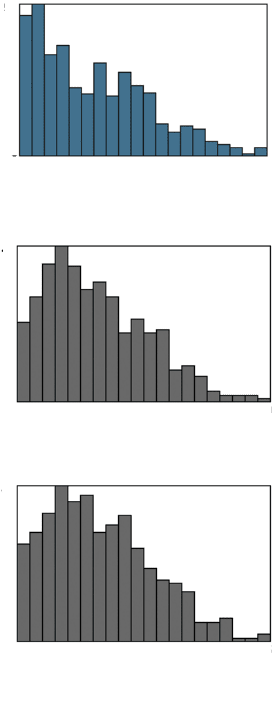
FIGURE 5.16

Size measurements on the cornstarch particles in Figure 5.1: (a) inscribed

circle; (b) circumscribed circle; (c) equivalent circular diameter.

Min = 1.00

Max = 17.41

To tal = 394, 20 bins

Mean = 6.29887, Std.Dev.=3.71002

Skew = 0.58911, Kurtosis = 2.75569

Count

Inscribed Radius

Min = 0.71

Max = 29.00

To tal = 394, 20 bins

Mean = 9.2432, Std.Dev.=5.76310

Skew = 0.61376, Kurtosis = 2.89793

Count

Circumscribed Radius

Min = 1.12

Max = 43.23

To tal = 394, 20 bins

Mean = 15.4848, Std.Dev.=9.04708

Skew = 0.52308, Kurtosis = 2.64997

Count

Equivalent Diameter

2241_C05.fm Page 300 Thursday, April 28, 2005 10:30 AM

measured in pixels) produce a plot that is skewed toward the right, but plotting

instead a histogram of the log values of the feature areas produces a Gaussian result.

The image in this example was processed by thresholding of the outlines of the

crystals, ﬁlling in the interiors, and applying a watershed segmentation.

But not all feature size distributions are Gaussian or log-normal. The cornstarch

particles shown in Figure 5.1 were measured using equivalent circular diameter,

inscribed circle radius, and circumscribed circle radius. The histograms (Figure 5.16)

do not have any easily-described shape, and furthermore each parameter produces

a graph with a unique appearance. It is not easy to characterize such measurements,

which often result when particle sizes and shapes vary widely.

COMPARISONS

When distributions have a simple shape such as a Gaussian, there are powerful

and efﬁcient (and well known) statistical tools that can be used to compare different

groups of features to determine whether they come from the same parent population

or not. For two groups, the student’s t-test uses the means, standard deviations and

number of measurements to calculate a probability that the groups are distinguish-

able. For more than two groups, the same procedure becomes the Anova (analysis

of variance). These methods are supported in most statistical packages and can even

be implemented in spreadsheets such as Microsoft Excel

For measurements that do not have a simple distribution that can be described

by a few parameters such as mean and standard deviation, these methods are inap-

propriate and produce incorrect, even misleading results. Instead, it is necessary to

use non-parametric statistical comparisons. There are several such methods suitable for

comparing groups of measurements. The Mann-Whitney (also known as Wilcoxon)

procedure ranks the individual measurements from two groups in order and calcu-

lates the probability that the sequence of groups numbers could have been produced

by chance shufﬂing. It generalizes to the Kruskal-Wallis test for more than two

groups. These methods are most efﬁcient for relatively small numbers of observations.

When large numbers of measurements have been obtained, as they usually are

when computer-based image analysis methods are employed, the ranking procedure

is burdensome. A much more efﬁcient technique for large groups is the Kolmogorov-

Smirnov (K-S) test. This simply compares the cumulative distribution plots of the

two groups to ﬁnd the greatest difference between them and compares that value to

a test value computed from the number of observations in each group. The probability

that the two groups do not come from the same population is then given directly.

Figure 5.17 illustrates the procedure for size data from two different groups of

measurements. The measurements of length have been replotted as cumulative

graphs, so that for each size the height of the line is the fraction of the group that

has equal or smaller values. In this speciﬁc case the horizontal axis has been

converted to a log scale, which does not affect the test at all since only the vertical

difference between the plots matters. The horizontal axis (the measured value) has

units, but the vertical axis does not (it simply varies from 0 to 1.0). Consequently,

the maximum difference between the two plots, wherever it occurs, is a pure number,

which is used to determine the probability that the two populations are different. If

2241_C05.fm Page 301 Thursday, April 28, 2005 10:30 AM

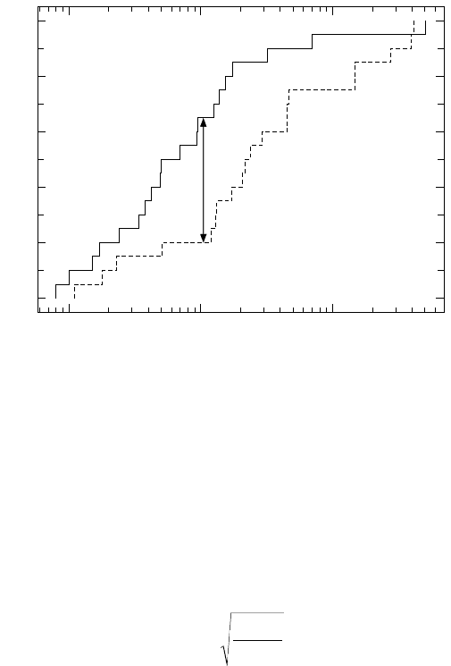
the difference value D is greater than the test value, then at that level of conﬁdence

the two groups of measurements are probably from different populations.

Tables of K-S test values for various levels of signiﬁcance can be found in many

statistical texts (e.g., D. J. Sheskin,

Parametric and Nonparametric Statistical Pro-

cedures

, Chapman & Hall/CRC, Boca Raton, FL, 2000), but for large populations

can be calculated as

(5.1)

where

and

are the number of measurements in each group, and

depends on

the level of signiﬁcance. For values of probability of 90, 95 and 99%, respectively,

takes values of 1.07, 1.22 and 1.52.

Other nonparametric tests for comparing populations are available, such as the

D’Agostino and Stephens method. The K-S test is widely used because it is easy to

calculate and the graphics of the cumulative plots make it easy to understand. The

important message here is that many distributions produced by image measurements

are not Gaussian and cannot be properly analyzed by the familiar parametric tests.

This is especially true for shape parameters, which are discussed below. It is con-

sequently very important to use an appropriate non-parametric procedure for statis-

tical analysis.

FIGURE 5.17

Principle of the Kolmogorov-Smirnov nonparametric test. The largest differ-

ence D that occurs between cumulative plots of the features in the two distributions is used

to compute the probability that they represent different populations.

0.1

1.0

10.0

Length (mm)

100

Cumulative Percent

=⋅

⋅

2241_C05.fm Page 302 Thursday, April 28, 2005 10:30 AM

EDGE CORRECTION

The measurements shown in Figures 5.15 and 5.16 were done with a correction

for edge-touching features. In the section above on counting, a procedure that

counted features intersecting two edges and ignored ones intersecting the other two

edges was used. But it is not possible to measure the features that intersect any edge,

because there is no information beyond the edge. Since large features are more likely

to intersect an edge than small ones, measurement and counting with no edge

correction would produce a biased set of measurements that systematically under-

represented large features. There are two solutions to this problem.

The older edge-correction procedure is based on the counting correction method.

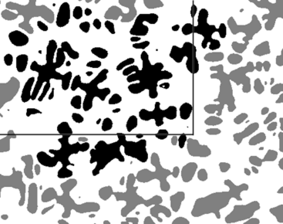
As shown in Figure 5.18, a guard region is drawn inside the image. Features that

cross the lines that mark the edge of the active counting region are measured and

counted normally, as are all features that reside entirely within the active region.

Features that lie inside the guard region are not measured or counted, nor is any

feature that touches the edge of the image. Consequently, the guard frame must be

wide enough that no feature ever crosses the edge of the active region (which requires

that it be measured and counted) and also reaches the edge of the image (which

means that it cannot be measured). That means the guard frame must be wider than

the maximum dimension of any feature present.

FIGURE 5.18

Use of a guard frame for unbiased measurement. The straight lines mark the

limits of the active measurement area. Features that lie in the guard frame region or intersect

any edge of the image are neither measured nor counted.

2241_C05.fm Page 303 Thursday, April 28, 2005 10:30 AM

Because the guard frame method reduces the size of active counting region

compared to the full image area, and results in not measuring many features that

are present in the image (because they lie within the guard frame), many computer-

based systems that work with digital images use the second method. Every feature

that can be measured (does not intersect any edge of the ﬁeld of view) is measured

and counted. But instead of counting in the usual way with integers, each feature is

counted using real numbers that compensate for the probability that other similar

features, randomly placed in the ﬁeld of view, would intersect an edge and be

unmeasurable.

As shown in Figure 5.19 and Equation 5.2, the adjusted count is calculated from

the dimensions of the ﬁeld of view and the projected dimensions of the feature in

the horizontal and vertical directions. For small features, the adjusted count is close to

1. But large features produce adjusted counts that can be signiﬁcantly greater than 1,

because large features are more likely to intersect the edges of the ﬁeld of view.

When distributions of feature measurements are plotted, the adjusted counts are used

to add up the number of features in each bin. Statistical calculations such as mean

and standard deviation must use the adjusted count as a weight factor for each

feature, complicating the math slightly.

(5.2)

The use of the adjusted count changes the shape of distributions slightly and

can markedly alter statistical values. Figure 5.20 shows the results for equivalent

circular diameter on the features within the entire image (not using a guard frame)

in Figure 5.18. Notice that the total count of features (ones that do not intersect any

FIGURE 5.19

When every feature within the image is measured, an adjusted count must be

used. The dimensions of the image (W

and W

) and the projected dimensions of the feature

and F

) are used to calculate the adjusted count according to Equation 5.2.

AdjCount

WFWF

XX YY

()()

⋅

−⋅−

2241_C05.fm Page 304 Thursday, April 28, 2005 10:30 AM

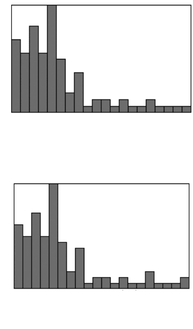
edge) is 92 without edge correction, but 106 with the correction, and the mean value

also increases by more than 10%.

As pointed out above, large features are more likely than small ones to intersect

the edge of the measuring ﬁeld so that they cannot be measured. Features whose

widths are more than 30% of the size of the image will touch an edge more often

than not. Note that it is absolutely not permitted to adjust the position of the camera,

microscope stage, or objects to prevent features from touching the edge. In general,

any ﬁddling with the ﬁeld of view to make the measurement process easier, or select

particular features based on aesthetic grounds, or for any other reason, is likely to

bias the data. There is a real danger in manual selection of ﬁelds to be measured.

The implementation of a structured randomized selection procedure in which the

opportunity for human selection is precluded is strongly encouraged to avoid intro-

ducing an unknown but potentially large bias in the results.

(a)

(b)

FIGURE 5.20

Effect of edge correction on the measurement data from the features in Figure

5.18: (a) without edge correction; (b) with edge correction.

Min = 1.95 Equivalent Diam.(cm) Max = 79.33

To tal = 92, 20 bins

Mean = 22.2584, Std. Dev. = 17.1842

Skew = 1.47378, Kurtosis = 4.64965

Count

Min = 1.95 Equivalent Diam.(cm) Max = 79.33

To tal = 106, 20 bins

Mean = 24.8842, Std. Dev. = 19.1968

Skew = 1.24078, Kurtosis = 3.63249

Count

2241_C05.fm Page 305 Thursday, April 28, 2005 10:30 AM

Edge intersection of large features can also be reduced by dropping the image

magniﬁcation so that the features are not as large. But if the image also contains

small features, they may become too small to cover enough pixels to provide an

accurate measurement. Features with widths smaller than about 20 pixels can be

counted, but their measurement has an inherent uncertainty because the way the

feature may happen to be positioned on the pixel grid can change the dimension by

1 pixel (a 5% error for something 20 pixels wide). For features of complex shape,

even more pixels are needed to record the details with ﬁdelity.

Figure 5.21 shows three images of milk samples. After homogenization, all of

the droplets of fat are reduced to a fairly uniform and quite small size, so selection

of an appropriate magniﬁcation to count them and measure their size variation is

straightforward. The ratio of maximum to minimum diameter is less than 5:1. But

before homogenization, depending on the length of time the milk is allowed to stand

while fat droplets merge and rise toward the top (and depending on where the sample

is taken), the fat is present as a mixture of some very large and many very small

droplets. In the coarsest sample (Figure 5.21c) the ratio of diameters of the largest

to the smallest droplets is more than 50:1.

It is for samples such as these, in which large size ranges of features are present,

that images with a very large number of pixels are most essential. As an example, an

image with a width of 500 pixels would realistically be able to include features up to

about 100 pixels in width (20% of the size of the ﬁeld of view), and down to about 20

pixels (smaller ones cannot be accurately measured). That is a size range of 5:1. But

to accommodate 50:1 if the minimum limit for the small sizes remains at 20 pixels and

the ﬁeld of view must be ﬁve times the size of the largest (1000 pixel) features, an

image dimension of 5000 pixels is required, corresponding to a camera of about 20

million total pixels. Only a few very high-resolution cameras (or a desktop scanner)

can capture images of that size. It is the need to deal with both large and small features

in the same image that is the most important factor behind the drive to use cameras

with very high pixel counts for microstructural image analysis.

Furthermore, a 50:1 size range is not all that great. Human vision, with its 150

million light sensors, can (by the same reasoning process) satisfactorily deal with

features that cover about a 1000:1 size range. In other words, we can see features

that are millimeter in size and ones that are a meter in size at the same time. To see

smaller features, down to 100

m for example, we must move our eyes closer to

the sample, and lose the ability to see large meter-size features. Conversely, to see

a 100 meter football ﬁeld we look from far off and cannot see centimeter size

features. So humans are conditioned to expect to see features that cover a much

larger range of sizes than digital cameras can handle.

There are a few practical solutions to the need to measure both large and small

features in a specimen. One is to capture images at different magniﬁcations, measure

them to record information only on features within the appropriate size range, and then

combine the data from the different magniﬁcations. If that is done, it is important to

weight the different data sets not according to the number of images taken, but to the

area imaged at each magniﬁcation. That method will record the information on indi-

vidual features, but does not include information on how the small features are spatially

distributed with respect to the large ones. For that purpose, it is necessary to capture

2241_C05.fm Page 306 Thursday, April 28, 2005 10:30 AM