Russ J.C. Image Analysis of Food Microstructure

Подождите немного. Документ загружается.

Measuring Features

Stereological techniques, introduced in Chapter 1, provide effective and efﬁcient

measurements of three-dimensional structures from images of sections through them.

Many of the procedures can be implemented using computer-generated grids com-

bined with binary images using Boolean logic, as shown in the preceding chapter.

Interpretation of the results is straightforward but assumes that proper sampling

procedures (e.g., isotropic, uniform and random probes) have been followed.

Another important task for computer-based image analysis is counting, measur-

ing and identifying the features present in images. This applies both to microscope

images of sections through structures, and to other classes of microscopic or mac-

roscopic specimens such as particles dispersed on a substrate. It is important to know

if the features seen in the images are projections or sections through the objects.

Projections show the external dimensions of the objects, and are usually easier to

interpret. Some section measurements can be used to calculate size information

about the three-dimensional objects as described in Chapter 1, subject to assumptions

about object shape.

COUNTING

For both section and projection images, counting of the features present is a

frequently performed task. This may be used to count stereological events (intersec-

tions of an appropriate grid with the microstructure), or to count objects of ﬁnite

size. This seems to be a straightforward operation, simply requiring the computer

program to identify groups of pixels that touch each other (referred to as “blobs” in

some computer-science texts). The deﬁnition of touching is usually that pixels that

share either a side or corner with any of their eight neighbors are connected. As

noted in the previous chapter, when this eight-connected convention is used for the

feature pixels, a four-connected relationship is implied for the background, in which

pixels are connected only to the four that share an edge.

For images in which all of the features of interest are contained entirely within

the ﬁeld of view, counting presents no special problems. If the result is to be reported

as number per unit area, the area of the image covered by the specimen may need

to be measured. But in many cases the image captures only a portion of the sample.

Hopefully it will be one that is representative in terms of the features present, or

enough ﬁelds of view will be imaged and the data combined to produce a fair

sampling of the objects. When the features extend beyond the area captured in the

image, there is a certain probability that some of them will intersect the edges of

the image. That requires a special procedure to properly count them.

2241_C05.fm Page 277 Thursday, April 28, 2005 10:30 AM

The simplest implementation of an unbiased counting procedure is to ignore

features that intersect two adjacent edges of the image (for instance, the right side

and the bottom) and to count features that reside entirely within the ﬁeld of view,

or are cut off by the other two edges. That produces an unbiased result because the

features that cross the right edge of this ﬁeld of view (and are not counted) would

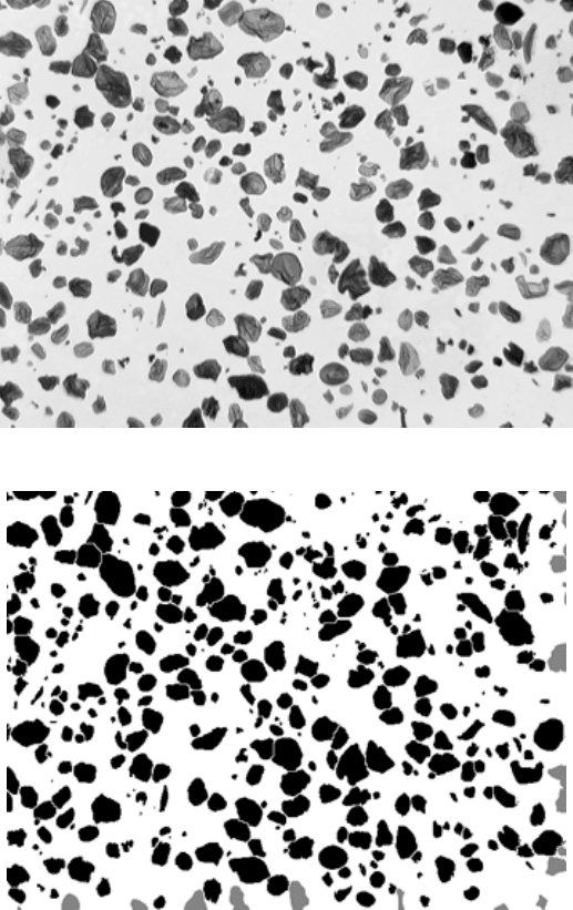
(a)

(b)

FIGURE 5.1

Example of unbiased feature counting: (a) cornstarch particles (courtesy of

Diana Kittleson, General Mills); (b) binary image after thresholding and watershed segmen-

tation. The light grey features are not counted because they intersect the bottom or right edges

of the image.

2241_C05.fm Page 278 Thursday, April 28, 2005 10:30 AM

cross the left edge of the next adjacent ﬁeld, and would be counted, and similarly

for the ones at the bottom. So the net count of features per unit area of the image

is unbiased and can be used as a representative estimate of the number of features

per unit area for the entire sample. Figure 5.1 illustrates this procedure. It is equiv-

alent (in a statistical sense) to counting features that cross any of the four edges of

the image as one-half.

If features are so irregular in shape (for instance, long ﬁbers) that they can cross

one of the edges where they should be counted, but can loop around and re-enter

the ﬁeld of view across one of the edges where they should not be counted, this

method won’t work correctly. In that case it is necessary to either ﬁnd a way (usually

a lower magniﬁcation image) to identify the features that touch the do-not-count

edges and avoid counting them where they reappear, or to ﬁnd some other unique

way to count features (such as the end points of ﬁbers, discussed in the preceding

chapter).

There are some situations in which other edge-correction methods are needed,

but they are all based on the same logic. For example, in counting the number of

pepperoni slices on one slice of pizza, features crossing one cut edge of the slice

would be counted and features crossing the other cut edge would not.

As discussed below, a more elaborate correction for edge effects is needed when

features are measured instead of just counted.

Measurement typically provides numerical information on the size, shape, loca-

tion and color or brightness of features. Most often, as noted above, this is done for

features that are seen in a projected view, meaning that the outside and outer

dimensions are visible. That is the case for the cornstarch particles in Figure 5.1,

which are dispersed on a slide. It is also true for the starch granules in Figure 5.2.

The surface on which the particles are embedded is irregular and tilted, and also

probably not representative because it is a fracture surface. The number per unit

area of particles cannot be determined from this image, but by assuming a regular

shape for the particles and measuring the diameter or curvature of the exposed

portions, a useful estimate of their size can be obtained. This is probably best done

interactively, by marking points of lines on the image, rather than attempting to use

automatic methods.

The image in Figure 5.2 illustrates the limited possibilities of obtaining mea-

surement information from images other than the ideal case, in which well dispersed

objects are viewed normally. Examining surfaces produced by fracture presents

several difﬁculties. The SEM, which is most conveniently used for examining rough

surfaces, produces image contrast that is related more to surface slope than local

composition and does not easily threshold to delineate the features of interest. Also,

dimensions are distorted both locally and globally by the uneven surface topography

(and some details may be hidden) so that measurements are difﬁcult or impossible to

make. In addition, the surface cannot in general be used for stereological measurements

because it hasn’t a simple geometrical shape. Planes are often used as ideal sectioning

probes into structures, but other regular surfaces such as cylinders can also be used,

although they may be more difﬁcult to image. Finally, the fracture surface is probably

not representative of the material in general, which is why the fracture followed a

particular path.

2241_C05.fm Page 279 Thursday, April 28, 2005 10:30 AM

These considerations apply to counting and measuring holes as well as particles.

Figure 5.3 shows another example of an SEM image of a fractured surface. Note

that in addition to the difﬁculties of delineating the holes in order to measure their

area fraction, that would not be a correct procedure to determine the volume fraction

using the stereological relationships from Chapter 1. A fracture surface is not a

random plane section, and will in general pass through more pores than a random

cut would intersect. Also, in this type of structure the large more-or-less round pores

are not the only porosity present. The structure consists of small sugar crystals that

adhere together but do not make a completely dense matrix, so there is additional

porosity present in the form of a tortuous interconnected network. The volume

fraction of each of these types of pores can be determined explicitly by measuring

the area fraction or using a point grid and counting the point fraction on a planar

section. However, from the SEM image it is possible to determine the average size

of the sugar crystals by autocorrelation as approximately 5.25

m, using the same

procedure as shown in Chapter 3, Figure 3.43

In Figure 5.4, the view of the ﬂat surface on which the particles reside is

perpendicular, but the density of particles is too high. Not only do many of them

touch (and with such irregular shapes, watershed segmentation is not a reliable

solution), but they overlap and many of the smaller particles hide behind the larger

ones. Dispersal of the particles over a wider area is the surest way to solve this

problem, but even then small particles may be systematically undercounted because

of electrostatic attraction to the larger ones.

For viewing particles through a transparent medium in which they are randomly

distributed, there is a correction that can be made for this tendency of small features

to hide behind large ones. Figure 5.5 illustrates the logic involved. The largest

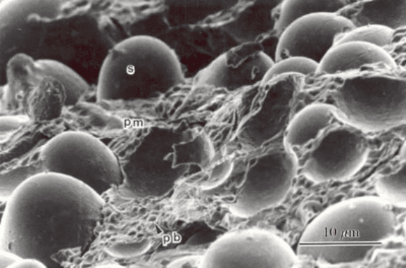
FIGURE 5.2

SEM micrograph of the fracture surface of a bean cotyledon. Starch granules

(S) are embedded in a protein matrix (pm). (Original image is Figure 3-23 in Aguilera and

Stanley, used with permission.)

2241_C05.fm Page 280 Thursday, April 28, 2005 10:30 AM

features can all be seen, so they are counted and reported as number per unit volume,

where the volume is the area of the image times the thickness of the sample. Then

the next particles in the next smaller class size are counted, and also reported as

number per unit volume. But for these particles, the volume examined is reduced

by the region hidden by the larger particles. For the case of a silhouette image, this

is just the area of the image minus the area of the large particles, times the thickness.

If smaller particles can be distinguished where they lie on top of the large ones, but

not behind them, then the correction is halved (because on the average the large

particles are halfway through the thickness). The same procedure is then applied to

each successive smaller size class. This method does not apply to most dispersals

of objects on surfaces because the distribution is usually not random, and the small

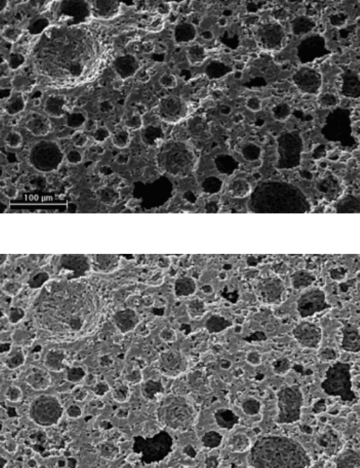
(a)

(b)

FIGURE 5.3

Scanning electron microscope image of the fractured surface of a dinner mint

(a). Retinex-based contrast compression (b) described in Chapter 3 makes it possible to see

the details inside the dark holes while retaining contrast in the bright areas. (Original image

courtesy of Greg Ziegler, Penn State University Department of Food Science.)

2241_C05.fm Page 281 Thursday, April 28, 2005 10:30 AM

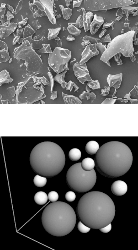
FIGURE 5.4

SEM image of pregelatinized cornstarch, showing small particles that are hid-

den by or adhering to larger ones.

FIGURE 5.5

Diagram of large and small particles in a volume.

2241_C05.fm Page 282 Thursday, April 28, 2005 10:30 AM

objects are much more likely to ﬁnd a hiding place under the large ones. There are

a few specialized sample preparation procedures that avoid this problem, in which

case the same correction procedure can be used, but usually the problem is solved

by dispersing the particles sufﬁciently to prevent overlaps.

Counting the number of features in an opaque volume requires the use of the

disector logic described in Chapter 1. The counting procedure can, of course, be

performed manually, but image processing routines can simplify the process as

shown in the following example. Figure 5.6 shows one cross section through an

aerated confection, obtained by X-ray tomography. In general such images show

density differences, and in this case the bubbles or voids are dark. A series of parallel

sections can be readily obtained by this approach, just as similar tomography (but

at a larger scale) is applied in medical imaging. From a series of such sections, a

full three-dimensional rendering of the internal structure can be produced, just as

from confocal microscope images or serial sections viewed in the conventional light

or electron microscope (except of course for the potential difﬁculties of aligning the

various images and correcting for distortions introduced in the cutting process).

Many different viewing modes, including surface rendering, partial transparency,

stereo viewing, and of course the use of color, are typically provided for visualization

of three-dimensional data sets, along with rotation of the point of view. Still images

such as those in Figure 5.7 do not fully represent the capabilities of these interactive

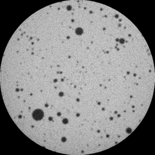
FIGURE 5.6

Tomographic cross-section of an aerated confection (courtesy of Greg Ziegler,

Penn State University Department of Food Science). The full width of the image is 14 mm,

with a pixel dimension of 27.34 µm.

2241_C05.fm Page 283 Thursday, April 28, 2005 10:30 AM

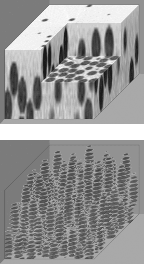
(a)

(b)

FIGURE 5.7

Examples of visualization of a small fragment of a three-dimensional data set

produced from sequential tomographic sections (note that the vertical dimension has been

expanded by a factor of 4 in these examples): (a) arbitrary surfaces through the data block;

(b) sequential sections with the matrix transparent, so that just the holes show; (c) surface

rendering of the holes with the matrix transparent.

2241_C05.fm Page 284 Thursday, April 28, 2005 10:30 AM

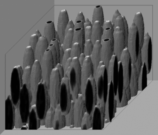
programs, but it should be emphasized that while the images have great user appeal,

and have become more practical with fast computers with large amounts of memory,

they are not very efﬁcient ways to obtain quantitative information. Indeed, few of

the three-dimensional visualization programs include signiﬁcant processing or mea-

surement tools.

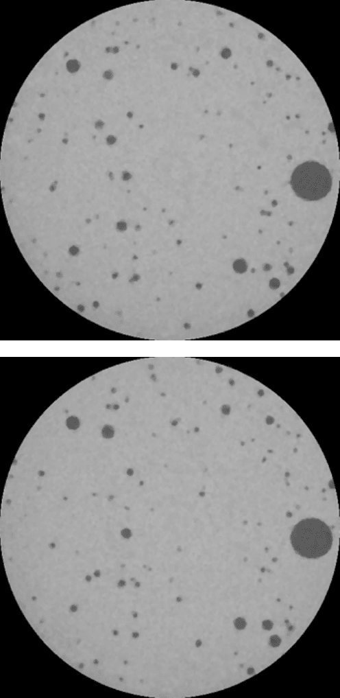
The disector logic presented in Chapter 1 requires a minimum of two parallel

images a known distance apart, such as those in Figure 5.8. Because the individual

sections are grainy (noisy) in appearance, processing was applied. The maximum

likelihood method introduced in Chapter 3 sharpens the brightness change at the

edges of the holes and reduces the grain in the image. making it easier to threshold

the holes. The disector count for convex features like these holes is simply the

number of intersections that are present in one section but not in both. The Feature-

AND logic presented in Chapter 4 identiﬁes the features present in both images (holes

that continue through both sections) even if they are different in size or shape. Removing

these features that pass through both section leaves those corresponding to holes for

which either end lies in the volume between the slices, which are then counted.

There are 65 features (intersections) counted, so the number of holes per unit

volume according to Equation 1.9 in Chapter 1 is 65/2 divided by the volume

sampled. That volume is just the area of the section image times the distance between

the sections, which is 9.7 mm

(6.3

m times 1.54 cm

). Consequently, N

is 3.35

holes per cubic millimeter. Since the area fraction of holes in a section can also be

measured (6.09%) to determine the total volume fraction of holes, the mean volume

of a hole can be determined as 0.0018 mm

. Of course, that measurement is based

(c)

FIGURE 5.7 (continued)

2241_C05.fm Page 285 Thursday, April 28, 2005 10:30 AM

(a)

(b)

FIGURE 5.8

Performing the disector count: (a, b) two sequential section images 63 µm apart,

processed with a maximum likelihood operator to sharpen the edges of the holes; (c) after

thresholding and Boolean logic, the binary image of the 65 holes that pass through either one

of the sections but not through both of them.

2241_C05.fm Page 286 Thursday, April 28, 2005 10:30 AM