Pump Handbook by Igor J. Karassik, Joseph P. Messina, Paul Cooper, Charles C. Heald

Подождите немного. Документ загружается.

2.32 CHAPTER 2

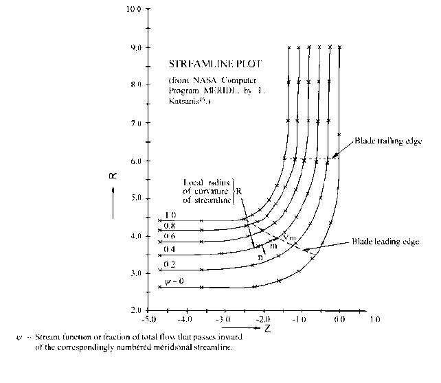
FIGURE 14 Axisymmetric flow analysis for the distribution of meridional velocity V

along the blade leading

edge (Eq. 51a)

shapes on the basis of fundamental fluid dynamical considerations, at the same time tak-

ing experience into account. Referring to Figure 13, an acceptable geometry can be

achieved by following these guidelines:

i. Maintaining the meridional flow area 2pr

b,1

at the blade leading edge at about the

same as it is at the eye, namely p(r

 r

), but then gradually increasing it versus

meridional distance to the generally larger value already established at the exit,

namely 2pr

ii. Choosing the minimum radius of curvature R

of the shroud to be about half the

radial opening at the eye.This avoids excessive local velocity V

1,sh

at the blade leading

edge.This has two consequences. Shaping the impeller blades to match a widely vary-

ing meridional approach velocity can complicate the construction of these blades. Also,

on first-stage impellers, if V

1,sh

is too great, the local pressure at that location will be

closer to the vapor pressure, increasing the required NPSH (or NPSH

). This is due

to a larger resulting value of the empirical factor k

, presented in Table 1 as the n

power of the velocity ratio V

1,sh

. Single-phase theory would require that the expo-

nent n  2, but two-phase activity in the pump reduces the local pressure reduction

that a single-phase application of Bernoulli’s equation would indicate.

Figure 14 is a plot of the meridional streamlines in the space between the hub and

shroud surfaces of the first-stage impeller of a high-energy boiler feed pump in the

absence of blades. This was obtained from a computer solution via Katsanis’ pro-

gram

of the inviscid axisymmetric flow field, which is governed by the following

equation:

2.1 CENTRIFUGAL PUMP THEORY 2.33

(51a)

As the average value of V

at the blade leading edge is about the same as its aver-

age V

in the eye, V

1,sh

can be estimated from the finite-difference form of this equation,

which expresses the change in V

from shroud to hub in terms of an average radius of

curvature R of the meridional streamlines across the passage of width n from shroud

to hub in the n-direction (normal to the streamlines in Figure 14):

(51b)

The estimated average R in Figure 14 is about twice the passage width n; so, by the

estimate of Eq. 51b, V

 . If half this difference is between V

and V

1,sh

, then

1,sh

 1.25. The computer solution of the inviscid axisymmetric-flow Eq. 51a in this

bladeless passage yields V

 0.73 and V

1,sh

 1.45 at this location

. Now, refer-

ring to Table 1, raising V

1,sh

to the power 1.4 would produce the typical value of 1.69

given for k

, which implies that the exponent n  1.4. However, two real effects oper-

ate to bias V

1,sh

toward lesser values; namely, a) greater loss of total pressure of

flow entering the impeller along the shroud

—

due to wall friction and higher velocity,

and b) shifting of the flow away from the shroud due to the presence of the impeller

blades, which in conventional designs present the incoming flow with the greatest

incidence at the hub. This serendipitous state of affairs tends to bring the value of n

back toward 2. Moreover, the above estimate of V

1,sh

 1.25 from Eq. 51b is more

typical of the flow for which designers tend to set the impeller blades at the inlet.

These results are strongly influenced by the radius of curvature at the shroud R

which in Figure 14 is about half of the passage width n. This accords with the guide-

line for R

iii. Shaping the hub profile compatibly with the guidelines as stated earlier. This is best

done after making an initial estimate of the shroud profile as outlined previously. The

distribution of meridional flow area from the eye to the exit should then be specified.

From this, a hub profile will emerge. As seen in Figures 13 and 14, the hub of a radial-

outflow impeller becomes essentially radial over the outer portion of its extent. If this

does not result from this procedure, appropriate adjustments can be made to the

shroud profile and the process repeated.

iv. For a high-specific-speed, axial-flow impeller, or inducer, the hub profile is often a cone

or a reverse curve between a smaller radial location at inlet to a larger one at outlet,

the latter radius decreasing with increasing specific speed as mentioned earlier. A

cone or cylinder for the shroud profile is often found in such machines.

e) Construction of the blades. The blades are designed by i) selecting the locus of the lead-

ing and trailing edges in the meridional plane, ii) establishing the surfaces of revolution

(streamwise lines in the meridional plane) from inlet to outlet along which the construc-

tion proceeds, iii) selecting the inlet angles, iv) selecting the outlet angles, v) establishing

the number of blades, and vi) obtaining the blade coordinates from inlet to outlet:

i. Leading and trailing edge loci. If every point along the leading and trailing edges is

revolved about the axis of rotation so as to lie in one meridional plane, the loci of these

edges appear as shown in Figure 13 or 14. The outer or shroud end of the blade lead-

ing edge is positioned at or near the minimum radial location; that is, at or near the

eye plane, whereas the inner or hub end is typically well back and largely around the

corner along the hub profile.These locations are desirable; first, at the shroud, because

the absolute velocity V (typically  V

) approaching the blade begins to decelerate

beyond the eye plane, so starting the blade ahead of this decelerating region tends to

¢V



¢n



2.34 CHAPTER 2

prevent separation of the fluid from the shroud surface due to the pumping action in

the blade channels

; and secondly, being far enough along the hub in the streamwise

direction to avoid impractical blade shapes (excessive twist, rake, and so on) that

would make both the construction and the flow inefficient. The locus of the blade trail-

ing edges is normally straight in the meridional plane and is axial in orientation for

most centrifugal pumps. At the higher specific speeds, this locus becomes more and

more slanted until it takes on the nearly radial orientation it has for a propeller (Fig-

ure 9).

ii. Surfaces of revolution for blade construction. Developing the coordinates of the

blades along three streamwise surfaces of revolution

—

the hub, mean, and shroud,

whose intersections with the meridional plane appear as streamwise lines in that

plane

—

usually provides a sufficient framework for shaping the blades of an impeller.

However, for high specific-speed impellers, where the passage width in the meridional

plane n (Figure 14) is large (about equal to or greater that the meridional distance

from leading to trailing edge), definition along two intermediate surfaces of revolution

is also needed to achieve a satisfactory design.

The “mean” line is one that is representative of the flow from a one-dimensional

standpoint as well as for the construction of the blades. Precisely, this is the mass-

averaged or “50%” streamline (that is, the streamline for c  0.5 in Figure 14)

—

which

evenly divides the mass flow

. This line is reasonably and conveniently approximated

by the “rms streamline;” that is, the line that would result in a uniform meridional

velocity distribution from hub to shroud and therefore equal areas 2prn normal to

the meridional velocity component V

. In this case, n (b) is the spacing between

the rms streamline and the hub or shroud line.This would put each point on the mean

line at the root mean square radial position along a true normal to the meridional

streamlines; hence, the “rms” terminology.

iii. Inlet blade angles. The blade angles are set to match the inlet flow field. This is done

where each of the previously chosen surfaces of revolution (that intersect the merid-

ional plane in the streamwise lines just described) crosses the chosen locus of the

blade leading edges in the meridional plane. At each such crossing point, an inlet

velocity diagram of the type shown in Figure 3 is plotted in a plane tangent to the sur-

face of revolution at that point. (Figure 3, representing a purely radial-flow configu-

ration, is a view of such a plane, as the surfaces of revolution are then simply disks.)

Each such velocity diagram or triangle contains a specific value of the angle b

f,1

between the relative velocity vector W

and the local blade speed vector U

r

The corresponding blade angle b

b,1

between the mean camber line of the blade and

the circumferential direction is set equal to b

f,1

or slightly higher than this to allow for

the higher V

m,1

caused by non-zero blade thickness at the leading edge and to allow for

higher flow rates that may be called for at off-design conditions. To construct the tri-

angle, one first plots U

and then V

m,1

, which is taken from an analysis such as that of

Figure 14 (altered as noted previously for the effect of the blades) or is chosen as the

mean value Q/2pr

b,1

(Figure 13) at the rms streamline. It is adjusted from experi-

ence at the shroud and hub. Likewise, if any prewhirl V

u,1

is delivered to the impeller,

it must be taken into account as illustrated in Figure 3.

iv. Outlet blade angles. Whereas the inlet velocity diagrams enable the designer to cor-

rectly set the blades to receive the incoming fluid with minimum loss, the outlet veloc-

ity diagram displays the evidence

—

through the magnitude of the circumferential

velocity component V

u,2

that the intended head will be delivered by the pump in accor-

dance with Eq. 15c. As shown in Figure 3, V

u,2

is determined

—

for the given impeller

tip speed U

—

by the exit relative flow angle b

f,2

in conjunction with the exit merid-

ional velocity component V

m,2

. This value of V

is somewhat larger than that given by

Eq. 16 because of a) blockage due to blade thickness and boundary layer displacement

thickness and b) the presence of any leakage flow Q

(Figure 2 and Eq. 11) that may

also be flowing through the impeller exit plane or Station 2.

Well inward of the exit plane, the direction of the one-dimensional relative velocity

vector W can be assumed to be parallel to the blade surface; however, in the last third

2.1 CENTRIFUGAL PUMP THEORY 2.35

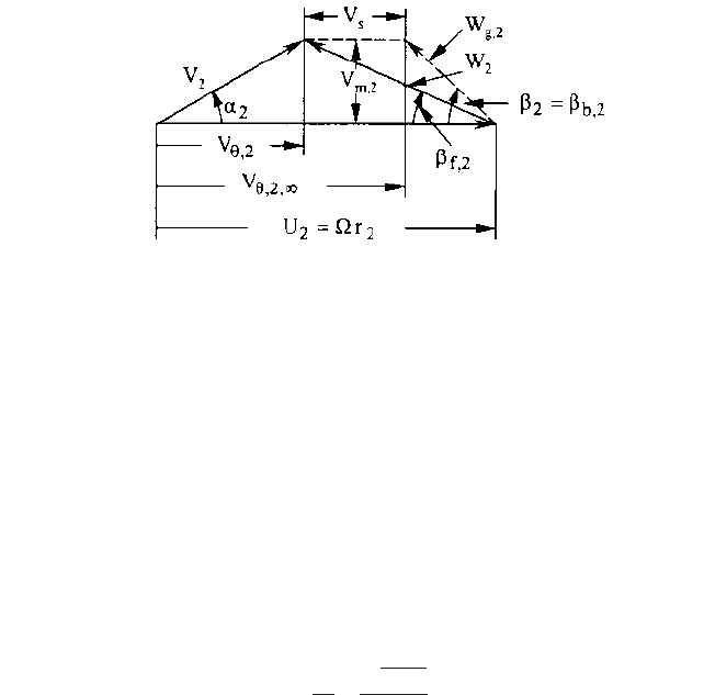
FIGURE 15 Impeller outlet velocity diagram

of the passage, the blade-to-blade distribution of the local relative velocity changes

due to the unloading of the blades at the exit. This produces a deviation of the direc-

tion of W

from that of the blade. This deviation, called “slip” in pumps, results in less

energy being delivered to the fluid by the impeller than would be the case if there were

“perfect guidance” such as would occur with an infinite number of blades.Accordingly,

in the outlet velocity diagram of Figure 15, the relative flow angle b

is less than the

blade angle b

. This deviation is quantified by the “slip velocity” V

. The magnitude of

depends on the distribution of loading along the blades from inlet to exit and there-

fore on the geometry of the flow passages and the number of blades. (Without slip, W

is the same as the “geometric” relative velocity W

g,2

shown in the figure.) The slip fac-

tor m  V

—

typically between 0.1 and 0.2

—

was determined theoretically by Buse-

mann for frictionless flow through impellers with logarithmic-spiral blades

(constant-b from inlet to exit) and a two-dimensional, radial-flow geometry with par-

allel hub and shroud

. Applicability of this theory to typical impellers, despite the dif-

ferences in geometry and the real fluid effects, was found to be good by Wiesner, who

represented Busemann’s results by the following convenient approximation

(52)

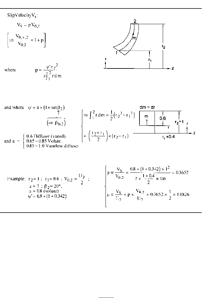
A broader, empirical slip correlation for pumps was developed by Pfleiderer, taking

into account impeller geometry and blade loading, as well as the influence of the down-

stream collecting system (volute or diffuser)

. Pfleiderer computes the slip velocity as

the product of a slip factor p and the impeller exit tangential velocity V

u,2

, where p is

computed as shown in Table 2. This table also contains a simple example; namely, a

radial flow impeller of a volute pump, for which the resulting value of m is 0.1826

—

versus 0.1498 via Eq. 52; however, in this case the latter result is low by about 15 per-

cent. A study of the Busemann plots in Wiesner’s paper yields m  0.18. Yet, if this had

been a vaned-diffuser pump, Pfleiderer would have predicted m  0.1468 for the same

impeller, as it would have delivered more V

u,2

for the same b

b,2

, W

g,2

, and, therefore, V

u,2

(Figure 15). This stems from the factor “a” in Table 2 having the value 0.6 (for a vaned

diffuser) instead of 0.8 (for a volute). So by this combination of circumstances

—

and in

this example

—

Eq. 52 describes the slip of a diffuser pump impeller. But, despite the

simplicity of Eq. 52, Pfleiderer’s method (Table 2) would appear to be a more rational,

comprehensive, and satisfying method for estimating slip in real pumps.

So, to find the outlet blade angle, the designer begins by deciding upon the required

value of V

u,2

; finds the exit flow angle and other elements of the diagram assuming the

existence of slip. Next, the designer computes the slip and then obtains the value of

the outlet blade angle b

b,2

. The process is iterative because the forementioned block-

age depends on the blade angle as well as the thickness.

m 



2sin b

0.7

2.36 CHAPTER 2

TABLE 2 Pfleiderer’s slip formula

v. Number of blades. The choice of the number of impeller blades is influenced by a)

interaction of the flow and pressure fields of the impeller and adjacent vaned struc-

tures such as the volute tongues or diffuser vanes and b) the need to maintain smooth,

attached

—

and therefore efficient

—

fluid flow within the impeller passages. The effect

of the number of blades on the interaction phenomenon is addressed in the latter part

of this section under the topic of high-energy pumps, where this issue becomes criti-

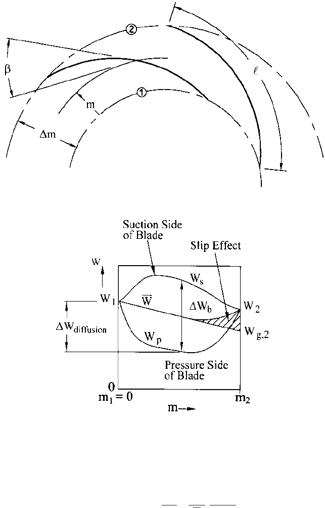
cal. Smooth, attached flow is assured if the product of the number of blades and their

total arc length / along a given meridional streamline, as illustrated in Figure 16, is

of sufficient magnitude. Divided by a representative circumference on that streamline,

usually that of the impeller outer diameter (OD), this product is called the solidity s:

(53)

In practice, solidity varies from about 1.8 at low specific speed (

 0.4 or N



1093) to slightly less than unity at 

 3 (N

 8199). For example, Dicmas’ curve

s 

 /

2pr

2.1 CENTRIFUGAL PUMP THEORY 2.37

FIGURE 17 Relative velocity distributions.

FIGURE 16 Intersection of impeller blades with mean surface of revolution

useful for 

 1 (N

 2733).This limits the relative velocity reduction that occurs on

the blade surfaces. Illustrated in Figure 17, this reduction or diffusion arises from the

loading on the blades expressed in terms of the blade-to-blade relative velocity differ-

ence W

(54)W

 W

1¢W

2

n



m, o

d1UV

2.38 CHAPTER 2

m,o

is the local meridional velocity component neglecting blockage. (One-dimension-

ally, V

m,o

is the value of V

found from Eq. 16, where the radius r is that from the axis

of rotation to the center of the circle of diameter b in Figure 8, which in turn lies on

an imaginary line in Figure 8 that is normal to the hub, shroud, and intermediate

stream surfaces.) Here, W

emerges by applying Bernoulli’s equation [Eq. 21 with no

change in radius (that is, no change in U) or loss as one traverses from pressure side

to suction side of the passage] to the static pressure difference p

 p

arising from the

delivery of angular momentum to the fluid (Eq. 26). This in turn results from the

application of the shaft torque to the blades. It is also assumed in the derivation of Eq.

54 that the blade-to-blade average relative velocity W lies halfway between the surface

velocities W

and W

, (which would exist just outside the boundary layers on the

blades,) as illustrated in Figure 17. This is a good assumption for efficient flow well

within a bladed channel

. W

is inversely proportional to the solidity because, on the

average, from inlet to outlet, Eq. 54 becomes

(55)

where it can be seen from Figure 16 and Eq. 53 that the fraction involving the num-

ber of blades n

is the reciprocal of the solidity s because

(56)

For unconventional impeller geometries, the foregoing solidity guidelines may be

inadequate to assure efficient flow. For any geometry, though, the concept of a diffu-

sion factor D, utilized by NACA researchers

to assess stationary cascades of airfoils

can be employed. In view of Eqs. 53

—

56, their equation for D takes the following form

for both axial- and non-axial-flow geometries, rotating or not:

(57)

This can be deduced from Figure 17 as follows:

(58)

Then, Eq. 57 is obtained through the definitions of the average value of W

(Eq. 55

with Eq. 56) and s (Eq. 53). NACA researchers found that losses increase rapidly if D

 0.6. However, many centrifugal pump impellers have virtually the same value of rel-

ative velocity W at in and at outlet

—

along the rms streamline (Figure 17), so D from

Eq. 57 is less than 0.6 on the rms streamline and even negative along the hub stream-

line. This situation was encountered in accelerating (turbine) cascades and led to the

use of local diffusion factors, one for each side of the blade, namely D

and D

. Here,

inspection of Figure 17 and Eq. 58 leads to

(59a and b)

where the 0.6 limit applies individually to D

and D

—

or to the sum of the two, in

which case the limit is 1.2. Eqs. 59a and 59b, therefore, constitute a more useful form

 1 

p, min

; D

 1 

s, max

D 

 W



¢W

a

¢W

diffusion

D  1 



¢ a

2sW

/  ¢m>sin b

 W

 ¢W

 a

2pr

sin b

¢m

b¢ a

2.1 CENTRIFUGAL PUMP THEORY 2.39

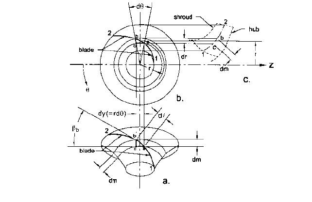
FIGURE 18 Blade construction: a) view of construction surface of revolution; b) polar view; c) meridional view

of the diffusion factor concept for assessing the blade loading and the choice of the

number of blades in centrifugal pump impellers

Finally, the total blade length or number of blades, should not exceed that necessary

to limit the diffusion as just described, as this adds unnecessary skin friction drag,

which causes a reduction in efficiency. Thus the solidity values given in conjunction

with Eq. 53 should not be appreciably exceeded, unless blade load needs to be reduced

to lower levels, as with inducers to limit cavitation

or impellers for pumps that must

produce lower levels of pressure pulsations.

vi. Development of the blade shape. Blades are developed by defining the intersection of

the mean blade surface (really an imaginary surface) or camber line on one or more

nested surfaces of revolution. Two such surfaces are formed by the hub and shroud

profiles. If the blade shape is two-dimensional (that is, the same shape at all axial

positions z), the mean blade surface is completely defined by constructing it on only

one such surface of revolution. Generally, however, the shape is three-dimensional and

is a fit to the shapes constructed on two or more of these surfaces of revolution;

namely, the hub and shroud and usually at least one surface between them. After this

final shape is known, half of the blade thickness is added to each side. (Sometimes the

full blade thickness is added to one side only, meaning that the constructed surface

just mentioned ends up

—

usually

—

as the pressure side of the finished blade rather

than the mean or “camber” surface. The effective blade angles are then slightly dif-

ferent from those of the pressure side used in the construction process.) The con-

struction along a mean surface of revolution is illustrated in Figure 18. The

distribution of the local blade angle b (or more precisely, b

) is found first by either the

“point-by-point” method or the conformal transformation method

—

both of which yield

the polar coordinates of the blade, r, u, and z. These coordinates also depend on the cho-

sen shapes of the intersections of the surfaces of revolution with the meridional plane;

that is, the hub, shroud, and mean meridional “streamline” or rms line, as in Figure

18c, and the fact that, on the surface of revolution Figure 18a, tan b  arc bc/arc ac 

dm/dy. The elemental tangential length dy ( arc ac) is the same on both the surface

of revolution (Figure 18a) and in the polar view (Figure 18b). From Figure 18b, it is

seen that dy  rdu, so the “wrap” angle u is found from

2.40 CHAPTER 2

(60)

and r and z are found from the fact that the coordinate m along each of the construc-

tion surfaces is a function of r and z (Figure 18c).

If the blade is two-dimensional, its mean surface consists of a series of straight-line

axial elements, each having a unique r and u at all z. Such a blade is typical of low-spe-

cific-speed, radial-flow impellers, and can be easily constructed by the “point-by-point”

method. Here, one specifies the distribution of W

—

often linear as in Figure 17

—

after

determining the hub and shroud profiles and the corresponding distribution of V

In effect, one obtains the distribution of the blade angle b

by constructing a velocity

diagram like the one in Figure 15 at every m-location from inlet (1) to outlet (2) in Fig-

ure 18c, dealing only with the “geometric” or non-deviated velocities, in order to get a

smooth variation of the blade angle b

vs m.Allowance is made for blockage due to the

thickness of the blades and the displacement thickness of the boundary layers in the

passage. The resulting wrap angle u for each m-point

—

as well as the corresponding r

and z

—

is then found from Eq. 60. (For convenience in designing the blades, the con-

struction angle u is often taken as positive as one advances from impeller inlet to exit.

For most impellers, this turns out to be opposite to the direction of rotation; and u is

taken in the direction of rotation for most other purposes of pump design and analy-

sis.) As discussed previously in Paragraph iv and illustrated in Figure 17, the actual

flow will deviate from the resulting blade via the “slip” phenomenon.

The point-by-point method allows the designer to exercise control over the relative

velocity distributions on the blade surfaces (Eq. 54 and Figure 17) via specification of

the distribution of W

or other velocity component in Figure 15; for example, V

. This

becomes more important if an unconventional impeller geometry is being developed

The point-by-point method can also be used for three-dimensional blades.A simple

approach in this respect would be to use this method to determine the blade shape

along the rms- or 50%-streamline (that is, on the mean surface of revolution depicted

in Figure 18).The shapes on the other streamlines, generally the hub and the shroud,

can also be found by this method. The resulting overall blade shape, however, is sub-

ject to the condition that the resulting wrap u

 u

cannot greatly differ on all

streamlines without the blade taking on a shape that is difficult to manufacture and

which may turn out to be structurally unsound or create additional flow losses. This

is because the final blade shape is the result of stacking the shapes that have been

established on the nested stream surfaces defined by these meridional streamlines.

Blade forces due to twists arising from this stacking could modify the expected flow

and cause unexpected diffusion losses.

One way to generate blade shapes along the hub and shroud that have the same

(or nearly the same) wrap as that obtained from point-by-point construction of the

blade on the mean surface of revolution is to establish the desired inlet and outlet

blade angles b

on each such surface and then mathematically fit a smooth shape

y(m) to these end and wrap conditions, where y is the tangential coordinate seen in

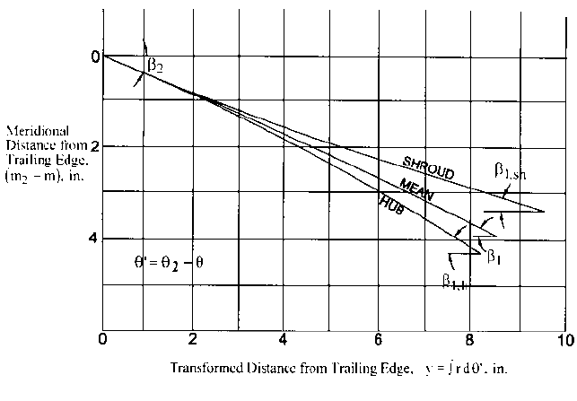
Figure 18 and defined in Figure 19. A conformal representation of the shapes of the

blades resulting from such a procedure on each of the three surfaces is seen in Fig-

ure 19. These shapes are sometimes called “grid-lines” or simply “grids”

—

from the

description of the graphical procedure that relates these shapes in the conformal

representation to those on the actual, physical surfaces

. In such a representation,

the blade angles are the same as they are on the physical surface of revolution

because tan b  dm/dy and dy  rdu, also yielding Eq. 60.

If the associated distributions of W

and V

are smooth, one can expect to have a sat-

isfactory result if these conformal representations are also smooth. Thus, many skilled

designers bypass the computations just described for the point-by-point method and

use the conformal transformation method of blade design. Here, one simply estab-

lishes the grid-line shapes by eye in the conformal plane of Figure 19, specifying the

blade angles b at inlet and outlet by the previous procedures as the starting point for

tan b



rdu

2.1 CENTRIFUGAL PUMP THEORY 2.41

FIGURE 19 Conformal transformation of blade shape: “grid-lines”

drawing each grid-line. This conformal blade shape is then transformed onto the phys-

ical surface, the differential tangential distance dy becoming rdu on the physical sur-

face (Figure 18) and the differential meridional distance dm being identical in both

the conformal and physical representations. If the resulting blade shape appears to be

unsatisfactory, the designer repeats this process, possibly first altering the hub and

shroud profiles or the blade leading and trailing edge locations on these profiles and

recomputing the b’s.

Designing the Collector The fluid emerging from the impeller is conducted to the

pump discharge port or entry to another stage by the collecting configuration, which can

employ one or more of the following elements in combination: a) volutes, which can be

used for designs of all specific speeds, b) diffuser or stator vanes, which are often more

economical of space in high-specific-speed single-stage pumps and in multistage pumps,

and for the latter, c) return or crossover passages, which bring the fluid from the volute

or diffuser to the eye of the next-stage impeller. Generally, the most efficient impeller has

a steady internal relative flow field as it rotates in proximity to these configurations.This

is assured by all of these elements because they are designed to maintain uniform static

pressure around the impeller periphery

—

at least at the design point or BEP. An excep-

tion to this rule is the concentric,“doughnut”-type, “circular-volute” collector, which is used

on small pumps or in special instances where the uniform pressure condition is desired

at zero flow rate.

The proximity of stationary vanes in these collecting configurations to the impeller must

be considered in their design. Called “Gap B,” the meridional clearance between the exit of

the impeller blades and adjacent vanes ranges from 4 to 15 percent of the impeller radius,

volutes having higher values in this range than diffusers, and pumps of higher energy level

requiring the larger values. If these gaps are too small, the interactions of the pressure fields

of the adjacent blade and vane rows passing each other can cause vibration and structural

failure of impeller blades, diffuser vanes, and volute tongues.

a) Volutes. A volute is built by distributing its cross-sectional area on a “base circle” that

touches the tongue or “cutwater” and is meridionally removed from the impeller exit by

Pump Handbook by Igor J. Karassik, Joseph P. Messina, Paul Cooper, Charles C. Heald - 3rd edition

Подождите немного. Документ загружается.