Pump Handbook by Igor J. Karassik, Joseph P. Messina, Paul Cooper, Charles C. Heald

Подождите немного. Документ загружается.

2.62 CHAPTER 2

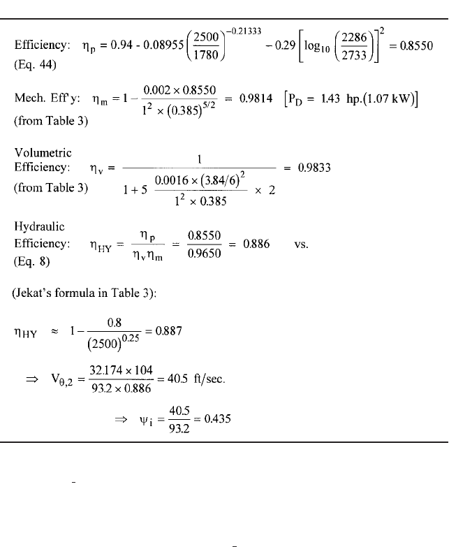
TABLE 9 Component efficiencies (design example)

 1.86)/sin(22 deg)  20.8 mm per blade, which for all six blades is 0.130 times the cir-

cumference of 37.7 in (958 mm). The width b

is computed to maintain V

m,2

at the chosen

value of 0.1715  U

, while accommodating this blockage and that of the sidewall bound-

ary layers. Altogether, it can be computed from these data that 85 percent of the merid-

ional exit area 2pr

is estimated to remain open for the one-dimensional flow of (Q  Q

)

at velocity V

m,2

, the boundary layers causing of the blockage. This is quite typical. An

openness of 90 percent is possible for larger impellers.

HUB-SHROUD PROFILES It is now possible, through the guidelines outlined in the discussion

of Figure 13, to finish plotting the hub and shroud profiles in Figure 25, which are also

seen in Figure 26c.At this point, the envelope of the leading edges of the blades is approx-

imated by a circular arc

—

later modified somewhat in the construction of the blades. The

arithmetic average radius of the meridional passage at the leading edges is found with

the circle of diameter 2.85 in (72.4 mm) to be 2.72 in (69.1 mm). The resulting line pass-

ing through the center of the circle is normal to both hub and shroud and is approximated

by the dashed straight-line leading-edge quasi-normal shown in the Figure 26c.

INLET VELOCITY DIAGRAMS The rms radial point on this quasi-normal line of Figure 26c

crosses the leading edges of the blades at r

1, mean

K r

1, rms

 2.91 in (73.9 mm) and is slightly

larger than the arithmetic average radius of 2.72 in (69.1 mm). It is this latter radius that

2.1 CENTRIFUGAL PUMP THEORY 2.63

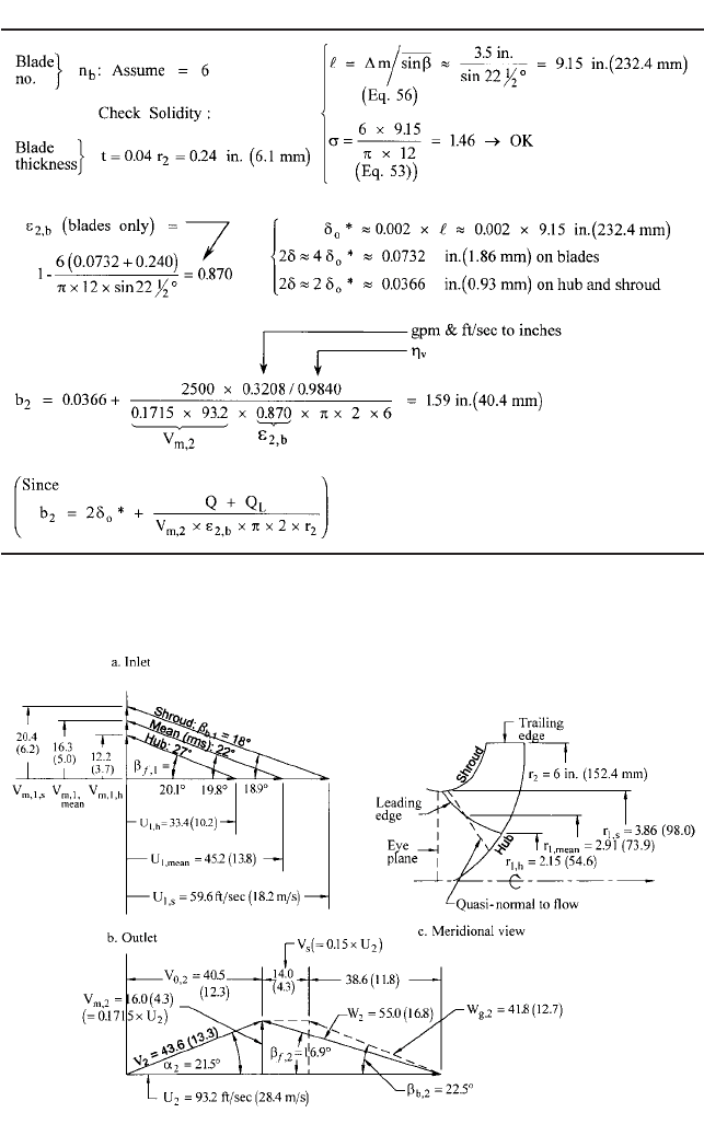
TABLE 10 Impeller blade blockage and width at exit (design example)

FIGURE 26A through C Impeller velocity diagrams for design example: a) inlet; b) outlet; c) meridional view

2.64 CHAPTER 2

must be used in computing the one-dimensional meridional velocity. After obtained, it is

applicable to the rms location (the location of the “mean” or “rms” inlet velocity diagram).

This diagram is one of three triangles shown for the inlet in Figure 26a, the other two

being located at the hub and shroud locations of the blade leading edges. Notice that V

m,1

for the rms triangle is 16.3 ft/sec (5.0 m/s), which is slightly less than the eye velocity V

of 17.3 (5.3). Allowing for blade blockage, this would bring the blocked meridional veloc-

ity V

within the blading closer to V

, the objective being to keep V

constant in the inlet

region and turn into the radial direction. The other triangles correspond to the radial loca-

tions of the blade at hub and shroud, as illustrated in Figures 26c and 27, and assume

that V

m,1,sh

 1.25 times V

m,1

, and V

m,1,h

 0.75 V

m,1

. A full Q3D solution would determine

these velocities more accurately; however, the design usually proceeds in this way

—

largely

because the hub blade angle is usually a good deal larger than hub flow angle. Efforts to

match the hub flow angle more closely entail special blading that is beneficial for high-

energy pumps but has little effect otherwise. The blade angle at the shroud is slightly

lower than the flow angle (by about 1 deg). This slightly negative incidence is actually

ideal for efficient flow and minimum cavitation. The largest values of U and W exist at

the shroud, as can be seen for the shroud inlet triangle, making it important to have the

best match at that point. Two deg positive incidence is quite common at the mean or rms

radial location and allows for blockage by the blades that does not increase the relative

velocity W as the fluid enters the impeller.

OUTLET VELOCITY DIAGRAM The outlet velocity components having been found in Tables 8

and 9, the slip velocity V

must still be found in order to obtain the complete outlet veloc-

ity diagram shown in Figure 26b. This slip is computed by Pfleiderer’s method (Table 2),

which utilizes the r(m) shape of the mean meridional streamline illustrated in Figure 27,

emerging as 15% of U

. The “a” factor for influence of the collector geometry was taken

in the middle of the range for volutes at 0.75; (see Table 2). Wiesner’s Eq. 52 yields 17.65%.

This would mean 6% less V

u,2

and head. However, this discrepancy is not unexpected, and

in view of the earlier discussions on slip, the Pfleiderer result is chosen as more realistic.

Nevertheless, uncertainty in the slip is the Achilles heel of the one-dimensional analy-

sis method. For this reason, most analysts “calibrate” their codes by deducing the slip from

test results and applying it to impellers of similar geometry. For Pfleiderer’s method, this

would be done by calibrating the “a” factor. CFD solutions now appear to be the best

approach to overcoming this difficulty.

As has been emphasized heretofore, this outlet velocity diagram contains the basic

information about the performance and design of the pump. It supplies the boundary con-

ditions for the volute design, but first the impeller blading that must produce it will be

established and evaluated.

IMPELLER BLADING

As indicated in Figure 26, the blade angles at both inlet and outlet

have been chosen at hub, mean, and shroud (with the same 22 deg all across the trailing

edge being assumed, although some would specify a little variation). Fitting a reasonable

blade shape between these end conditions can be done in the conformal plane (illustrated

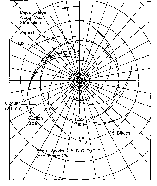
in Figure 19). These shapes, when transformed as described earlier, yield the hub, mean,

and shroud blade shapes identified in the polar view of Figure 28. In actuality, the inverse

“point-by-point” method was used, specifying W

as indicated in Figure 29 and, at each of

the 21 stations along the mean line of Figure 27, developing the velocity diagrams in the

manner employed to arrive at Figure 26b; obtaining b

at each station; and developing the

mean-streamline blade shape of the polar view with Eq. 60. Involved in this procedure

—

which was computerized

—

was the calculation at each station of the blockage and of the

local slip velocity, the latter being estimated as a fraction of the discharge slip velocity V

that increases rapidly to unity as the exit is approached.

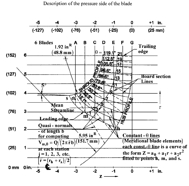
Note that the meridional area is needed at each station in order to compute V

. As indi-

cated in Figure 27, this is approximated here as the area of the frustum of a cone defined

by the dashed lines or “quasi-normals,” which are as nearly perpendicular to both hub and

shroud as possible. Except for some machines with meridionally curved passages and a

large passage width-to-length ratio causing the true normals to be strongly curved, the

quasi-normal approach works well.

2.1 CENTRIFUGAL PUMP THEORY 2.65

FIGURE 27 Impeller blading–meridional view (design example)

To establish the blade shapes along the hub and shroud, the corresponding “grid lines”

of Figure 19 were found from polynomials satisfying the end conditions of blade angle and

location, the y-position of the inlet end of the grid line being iterated until the desired

blade wrap was obtained. In this way, different wrap angles u ( u

 u

) can be imposed,

but a tolerable resulting blade shape requires that these us be not much different from

the u ( 119.1 deg) obtained on the mean line from the method just described. In this

example, it was possible to maintain u the same on all three construction lines. Alterna-

tively and perhaps more consistently, the inverse approach could be applied at hub and

shroud as well as on the mean line.

Regardless of which procedure is used to generate the hub, mean and shroud blade

shapes

—

the conformal transformation method, the point-by-point method, or some combi-

nation

—

the shape of the blade everywhere else still needs to be established. To do this, the

shapes of the constant-u lines in Figure 27

—

called “blade elements”

—

must be specified.This

can be done mathematically as indicated on the figure or by eye (the latter approach is

widely used). Note that each constant-u line actually lies in a different meridional plane.

Thus, Figure 27 depicts a superposition of all 21 meridional planes, each containing an inter-

section of the blade surface and appropriately identified as having the u-value noted on the

figure.

DIFFUSION ASSESSMENT Figure 29 is a presentation of the free-stream relative velocity dis-

tributions at the blade surfaces and halfway between. The rapid approximate method of

2.66 CHAPTER 2

FIGURE 28 Impeller blading—polar view, showing pressure sides of the blades (design example)

Stanitz (Eq. 54) is utilized to obtain the surface W’s, the mean values of W on the mean

(rms) streamline coming from the local velocity diagrams developed at each station

. The

mean W’s at hub and shroud are found at the ends of the respective constant-u lines under

the assumption that the ideal head or UV

-product is constant along each of these lines

from hub to shroud. This is usually a fair approximation; however, a Q3D analysis (Fig-

ure 14) would yield a closer estimate of these mean W-distributions

16,41

. Nevertheless, the

diffusion factors computed from the plotted surface velocities by means of Eqs. 59 are

shown on the figure

—

these values are well below the 0.6 limit. This would indicate that

the resulting solidity of 1.48 (originally estimated at 1.46 in Table 10) is adequate, and

that the correct number of blades was chosen.

Notice also on Figure 29 that the exit value of W is significantly larger than W

, which

is consistent with the outlet velocity diagram of Figure 26b. Further, a slight jump in the

mean W at the inlet is indicated; however, as the higher value of W is not sustained, it is

2.1 CENTRIFUGAL PUMP THEORY 2.67

FIGURE 29 Blade surface relative velocity distributions (design example)

unlikely that it actually occurs in the 3D velocity field. Moreover, details near leading and

trailing edges are not well handled by Eq. 54

—

a 2D blade-to-blade solution is more desir-

able for this type of diffusion assessment

Volute Design With the exit velocity V

of 43.6 ft/sec (13.3 m/s) and the tangential veloc-

ity component V

u,2

of 40.5 ft/sec (12.3 m/s) from Figure 26b, the volute design process is

started in Table 11 using Eq. 61. This entails a choice of the radial “Gap B” of 6% of the

impeller radius r

and a tongue leading edge thickness t

equal to 70 percent of the

impeller blade thickness. These choices are not critical for a pump of low energy level such

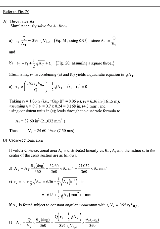
as this is, as the stresses imposed by the flow on structural elements are small. The throat

area A

is then found to be 32.60 in

(21,032 mm

) and the throat velocity V

computes to

24.60 ft/sec (7.50 m/s), which is 56% of V

and so represents considerable diffusion from

impeller exit to throat. (The throat area A

is the fundamental feature of a volute and acts

in concert with the impeller exit area, as emphasized by Anderson

and Worster

and

described in the earlier part of this section on Designing the Collector in terms of the inter-

section of the casing and impeller lines

2.68 CHAPTER 2

TABLE 11 Volute casing (design example)

The circumferential distribution of the volute cross-sectional area A

versus polar angle

from the tongue (Figure 20a) is developed in the latter part of Table 11, a final listing

being presented for a) linear A

versus u

and b) constant one-dimensional angular

momentum r

. This listing illustrates an earlier statement that the latter approach pro-

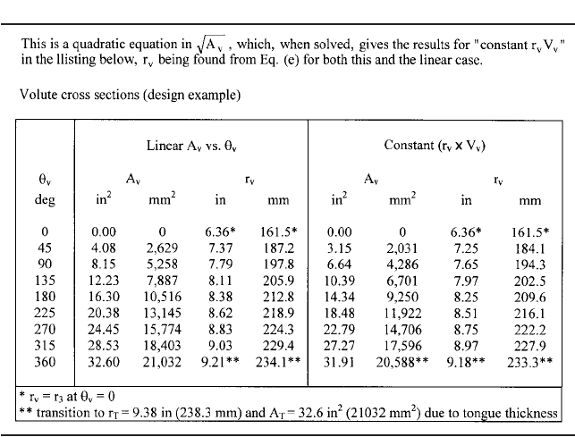
2.1 CENTRIFUGAL PUMP THEORY 2.69

TABLE 11 Continued.

duces smaller areas upstream of the throat than does the former. Frictional effects in the

smaller-A

portion of the volute are less prominent using the linear approach. A CFD

assessment at all flow rates can be made to guide the design choice here. Finally, the one-

dimensional constant r

method can be improved upon by integrating a constant rV

dis-

tribution over each cross section, and the proper design must satisfy also continuity

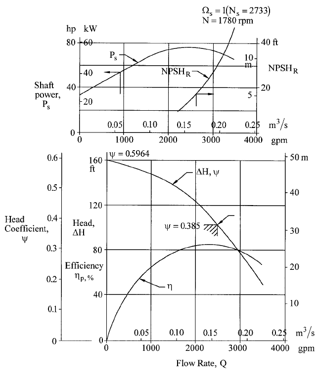
Estimated Performance Characteristics Detailed computation of hydraulic losses,

together with leakage, disk friction, and other mechanical drags was done as described pre-

viously, and the results are presented in Figure 30.The method predicts the pump efficiency

to be 85.5% at the design point of 2500 gpm (0.1577 m

/s), peaking at 86 percent at a 5%

lower flow rate. The power consumption peaks at the design point at 77 hp (57 kW), indi-

cating that this is a “non-overloading” design; that is, shaft power does not increase beyond

this flow rate. The empirical methods reviewed earlier for shut-off head and power were

applied here and blended into the one-dimensionally computed curves at half of the BEP

flow rate.

The shut-off head coefficient value of 0.596 is close to the 0.585 value of Stepanoff

and

is admittedly open to alteration. The rise of head from design point to shut-off is from 104

up to 161 ft (31.7 up to 49.1 m) or 55%. This percentage could be smaller and still ensure

stable operation in any typical system; however, the non-overloading feature could change,

the power peaking at a higher flow rate. In retrospect, the design-point head coefficient c

of 0.385 could be larger without the diffusion-factor results of Figure 29 becoming exces-

sive. One would conclude from this exercise that the c-curve of Figure 12 is conservative

and could be higher. Of more significance, however, is the demonstration in this design

example of the utilization of easily applied fundamental fluid dynamical analyses such as

the diffusion assessment illustrated in Figure 29 as the basic arbiters of design choices

such as the head coefficient, number of blades, and so on. Furthermore, the shapes of the

performance characteristics are revealed.

2.70 CHAPTER 2

FIGURE 30 Estimated performance characteristics (design example)

The shut-off power is 34 hp (25 kW), arising from a power coefficient of 0.047 from

Mockridge’s correlation

for a b

of 1.59/12 ( 40.4/304.8)  0.1325

—

as found from

Figure 23. This is 44% of the design-point power, a typical result. As seen in Section

2.3.1, this percentage increases with specific speed, where, of course, b

is also

larger

The NPSHR ( NPSH

for this example) at off-design conditions is estimated empir-

ically. At the higher, non-recirculating flow rates, NPSHR is related to the head required

to accelerate the relative velocity within the blades to values higher than at the design

point

. As stated in Section 2.3.1, operation at NPSH

involves performance in the pres-

ence of extensive internal two-phase behavior. This is complicated by recirculation at the

lower flow rates. Therefore, the full NPSHR curve in such a case usually has to be estab-

lished experimentally.

2.1 CENTRIFUGAL PUMP THEORY 2.71

HIGH-ENERGY PUMPS ________________________________________________

Over the past few decades, there has been a trend toward pumping machinery that con-

centrates more power within a given volume. This trend is driven by cost and technology

improvements. The basic energy transfer relationships show that smaller size demands

higher rotative speed. Thus, over the same time period, speeds of high-power pumps have

been increasing. Moreover, the number of stages in multistage pumps has been decreas-

ing. There have been spikes in these trends; the resulting pumps suffering from excessive

vibration, rotor and hydraulic instabilities, component failure, and cavitation damage

The term “high energy” has been applied to these machines, and this label can be quanti-

fied in terms of the stresses arising in critical pump components and the likelihood of an

adverse mechanical response that such stress levels imply. Research has led to technical

solutions for effectively controlling rotordynamic behavior and reducing unsteady

hydraulic thrust and surge as well as cavitation erosion

53,58,59

. The resulting pump relia-

bility improvements and life extension should enable the previous trends to continue.

Being aware of the energy level enables the pump user to assess whether operation and

maintenance difficulties are likely to occur after the pump is installed and running, and it

enables the designer to take the appropriate measures to ensure the technical integrity of

the product.

Pressure Pulsations Measured at the inlet or outlet port, the amplitude of the pres-

sure pulsations can be a significant fraction of the pressure rise of the pump

—

especially

at flow rates well below that of the BEP for the speed involved. Sources are a) the inter-

action of the pressure fields of the impeller and diffuser or volute, b) unsteady separated

and reversed flows at impeller inlet and discharge and in the diffuser, c) cavitating flows,

and d) combinations of these phenomena. Pressure pulsations presumed to exist at the

impeller OD from the interaction of impeller blade-to-blade and diffuser vane-to-vane

variations of pressure have been calculated by inviscid flow analysis to have a peak-to-

peak amplitude that is of the same order as the static pressure rise of the impeller

. More-

over, the viscous, thicker wakes existing at lower-than-BEP flow rates (here called “low

flows”) and separated recirculating fluid from both impeller and diffuser that participate

in these interactions can be expected to increase the pressure pulsation amplitude at such

conditions.

Figure 31 confirms these ideas, showing a bronze impeller that operated extensively at

low flow. Cavitation pitting can be observed near the OD of the impeller, which means that

the rarefactions of the pressure waves were below the vapor pressure of the liquid

—

these

pressure minima therefore being below the inlet pressure to the impeller. Moreover, the

bulged-out shrouds can be assumed to be the result of the repeated occurrence of the asso-

ciated pressure spikes (that is, the maxima of the pressure waves) within the radial gap

(“Gap B”) between the impeller blades and the diffuser vanes, the sidewall pressures on the

outsides of the shrouds remaining comparatively constant.At greater values of design pres-

sure rise than was the case for this impeller, this phenomenon creates correspondingly

greater forces that have led to actual breakage of the impeller shrouds and diffuser vanes

The cavitation seen in Figure 31, can also be observed on the leading edges of diffuser vanes,

as in Figure 21 of Section 9.5, and this raises the possibility of diffuser vane breakage.

Energy Level: Stage Pressure Rise Even in the absence of the weakening effect of

cavitation erosion, the leading edge of a diffuser vane or volute tongue is a representa-

tive, highly stressed zone within a pump that is subject to failure if the magnitude of the

pressure pulsations arising from the impeller-diffuser interactions just described is suffi-

ciently large. Thus, the hydraulically induced stresses in these vanes can be the basis for

quantifying the energy level of a pump stage. In Table 12, this concept is developed into

an expression for the stress in terms of the fluctuating pressure magnitude dp that is

assumed to act across the vane leading edge as illustrated in the table. The width b of the

vane is close enough to b

of the impeller exit to utilize the relationships for c and f

Figure 12 to relate b/D to specific speed in Eq. (c) of the table. For similar velocity fields,

the pressure pulsation magnitude dp is a constant multiplied by the stage pressure rise

P

stg

. Thus, for a limiting value of stress, the concept of a limiting stage pressure rise

Pump Handbook by Igor J. Karassik, Joseph P. Messina, Paul Cooper, Charles C. Heald - 3rd edition

Подождите немного. Документ загружается.