Klir G.J. Uncertainity and Information. Foundations of Generalized Information Theory

Подождите немного. Документ загружается.

Hence S(X ¥ Y ) £ S(X) = S(Y ); and furthermore (again by Gibbs’ theorem),

the equality holds if and only if

which means that the random variables whose state sets are X and Y are

noninteractive. 䊏

Theorem 3.4 can easily be generalized to more than two sets. Its general

form is

(3.39)

which holds for every n Œ ⺞.

Theorem 3.5

(3.40)

Proof. From Theorem 3.3,

and from Theorem 3.4

Hence,

and the inequality

follows immediately. 䊏

Exchanging X and Y in Theorem 3.5, we obtain

Additional equations expressing the relationships among the various

entropies and the information transmission can be obtained by simple formula

SY SY X

()

≥

()

SX Y SX

()

SX Y SY SX SY

()

SX Y SX SY¥

()

SX Y SX Y SY

()

=¥

()

SX SX Y

()

≥

()

SX X X SX

¥¥¥

()

...

px y p x p y

()

◊

()

82 3. CLASSICAL PROBABILITY-BASED UNCERTAINTY THEORY

manipulations with the aid of key properties in Theorems 3.3 through 3.5. For

example, when we substitute for S(X, Y) from Eq. (3.35) into Eq. (3.34), we

obtain

(3.41)

similarly, by substituting Eq. (3.36) into Eq. (3.34), we obtain

(3.42)

By comparing Eqs. (3.41) and (3.42), we also obtain

(3.43)

For each type of the Shannon entropy, S, the normalized counterpart, NS,

is calculated by dividing the respective entropy by its maximum value. Thus,

for example,

(3.44)

(3.45)

(3.46)

The range of each of these counterparts is, of course, [0, 1]. The maximum

value, T

(X, Y), of information transmission associated with joint probability

distributions on X ¥ Y can be derived in a similar way as its possibilistic coun-

terpart (Eq. (2.34)). It is given by the formula

(3.47)

Then,

(3.48)

3.2.4. Examples

The purpose of this section is to illustrate the various properties and applica-

tions of the Shannon entropy by simple examples, some of which are proba-

bilistic counterparts of examples in Chapter 2.

NT X Y

TXY

()

, min log ,log .TXY X Y

()

{}

NS X Y

SX Y

()

log

NS X Y

SX Y

()

◊

()

log

NS X

()

log

SX SY SX Y SY X

()

TXY SY SYX

()

TXY SX SXY

()

3.2. SHANNON MEASURE OF UNCERTAINTY FOR FINITE SETS 83

EXAMPLE 3.2. Consider two variables, X and Y, whose states are 0 or 1 and

whose joint probabilities p(x, y) on X ¥ Y = {0, 1}

are speciﬁed in Table 3.1a.

Uncertainty associated with these joint probabilities is determined by the

Shannon entropy

The marginal probabilities p

(x) and p

(y), calculated by Eqs. (3.5) and (3.6),

are shown in Table 3.1b. Their uncertainties are:

The conditional uncertainties can now be calculated by Eqs. (3.35) and (3.36):

Moreover, the information transmission, which expresses the strength of the

relationship between the variables, can be calculated by Eq. (3.34):

EXAMPLE 3.3. Consider the same variables as in Example 3.2. However,

only their marginal probabilities given in Table 3.1b are known.Assume in this

TXY SX SY SXY

,..

()

-¥

()

= 019

SX Y SX Y SY

SY X SX Y SX

()

=¥

()

=¥

()

028

069

()

=- - =

()

=- - =

09 01 01 01 047

07 07 03 03 088

. log . . log . . ,

. log . . log . . .

SX Y¥

()

=- - - =07 07 02 02 01 01 116

222

. log . . log . . log . . .

84 3. CLASSICAL PROBABILITY-BASED UNCERTAINTY THEORY

Table 3.1. Illustration to Example 3.2

xy p(x, y)

0 0 0.7

0 1 0.2

1 0 0.0

1 1 0.1

(a)

(x) yp

(y)

0 0.9 0 0.7

1 0.1 1 0.3

(b)

xyp

(x)·p

(y)

0 0 0.63

0 1 0.27

1 0 0.07

1 1 0.03

(c)

example that the variables are independent. Since probabilistic independence

is equivalent to probabilistic nonineteraction, as shown in Section 3.1.1, we can

calculate their joint probability distribution based on this assumption by Eq.

(3.7). This joint distribution is shown in Table 3.1c. The uncertainty, S

ind

, based

on the assumption of independence is thus readily calculated as

Observe that S

ind

(X ¥ Y ) - S(X ¥ Y ) = 0.19. This means that 0.19 bits of infor-

mation are gained when we know the actual joint probability distribution in

Table 3.1a.

EXAMPLE 3.4. Consider three variables, X, Y, Z, whose states are in sets X

= Y = {0, 1} and Z = {0, 1, 2}, respectively. The joint probabilities on X ¥ Y ¥ Z

are given in Table 3.2a. In this case, there are six distinct conditional uncer-

tainties and four distinct information transmissions.To calculate them, we need

SXY

ind

()

=- -

-- =

063 063 027 027

007 007 003 003 135

. log . . log .

. log . . log . . .

3.2. SHANNON MEASURE OF UNCERTAINTY FOR FINITE SETS 85

Table 3.2. Illustration to Example 3.4

xyzp(x,y,z)

0 0 0 0.05

0 1 0 0.10

0 0 2 0.22

1 0 0 0.05

1 0 1 0.20

1 0 2 0.10

1 1 1 0.08

1 1 2 0.20

(a)

xyp

(x,y)

0 0 0.27

0 1 0.10

1 0 0.35

1 1 0.28

xzp

(x,z)

0 0 0.15

0 2 0.22

1 0 0.05

1 1 0.28

1 2 0.30

yzp

(y,z)

0 0 0.10

0 1 0.20

0 2 0.32

1 0 0.10

1 1 0.08

1 2 0.20

(x)

0 0.37

1 0.63

(y)

0 0.62

1 0.38

(z)

0 0.20

1 0.28

2 0.52

S(X ¥ Y ¥ Z) = 2.80 S(X ¥ Y) = 1.89 S(X) = 0.95

S(X ¥ Z) = 2.14 S(Y) = 0.96

S(Y ¥ Z) = 2.41 S(Z) = 1.47

(d)

(b)

(c)

to determine all two-variable marginal probability distributions (shown in

Table 3.2b) and all one-variable marginal probability distributions (shown

in Table 3.2c). Values of the Shannon entropy for all probability distributions

in Table 3.2(a)–(c) are shown in Table 3.2d. These values form the basis from

which all the conditional uncertainties and information transmissions are

calculated as follows:

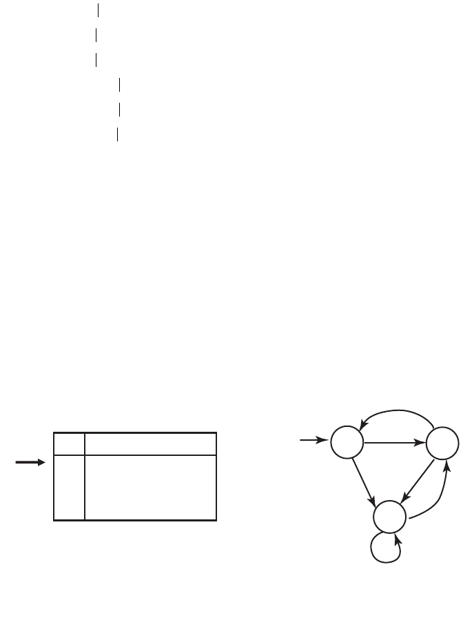
EXAMPLE 3.5. This example is in some sense a probabilistic counterpart of

the simple nondeterministic dynamic system discussed in possibilistic terms

in Examples 2.1 and 2.2. The subject here is a simple probabilistic dynamic

system with state set X = {x

, x

}. State transitions of the system occur only

at speciﬁed discrete times and are fully determined for each initial probabil-

ity distribution on X by the conditional probabilities speciﬁed by the matrix

or the diagram in Figure 3.3a and 3.3b, respectively.

SX Y Z SX Y Z SY Z

SY X Z SX Y Z SX Z

SZ X Y SX Y Z SX Y

SX Y Z SX Y Z SZ

SX Z Y SX

()

=¥¥

()

-¥

()

=¥¥

()

-¥

()

=¥¥

()

-¥

()

=¥¥

()

=¥

039

066

091

133

YYZ SY

SY Z X SX Y Z SX

TX YZ SX Y SZ SX Y Z

TX ZY SX Z SY SX Y Z

TY Z X SY

()

=¥¥

()

=¥

()

-¥¥

()

=¥

()

-¥¥

()

184

185

056

030

, ¥¥

()

-¥¥

()

-¥¥

()

ZSXSXYZ

TX YZ SX SY SZ SX Y Z

056

058

,..

86 3. CLASSICAL PROBABILITY-BASED UNCERTAINTY THEORY

0.0 0.9 0.1

0.2 0.0 0.8

0.0 0.6 0.4

= M

(a)

(b)

Next states

Present states

0.2

0.9

0.1

0.8

0.6

0.4

Figure 3.3. Simple probabilistic system discussed in Example 3.5.

To describe how the system behaves, let t = 1,2,...denote discrete times

at which state-transitions occur, let p(

) denote the probability of state x

time t, and let

denote the probability distribution of all states of the system at time t. Fur-

thermore, let M = [m

] denote the matrix of conditional probabilities

t+1

) for all pairs ·x

, x

ÒŒX

, which are independent of t. That is,

for all i, j Œ ⺞

and all t Œ⺞.

Given the probability distribution

p at some time t, the system is capable

of predicting probability distributions at time t + k (k = 1, 2, . . .) or probabil-

ity distributions of sequences of future states of some lengths. The Shannon

entropy of each of these distributions measures the amount of uncertainty in

the respective prediction.We can also measure the amount of information con-

tained in each prediction made by the system (predictive informativeness of

the system). For each prediction type, this is the difference between the

maximum predictive uncertainty allowed by the framework of the system and

the actual predictive uncertainty. The maximum predictive uncertainty is

obtained for the state-transition matrix, M

= [mˆ

], in which each row is a

uniform probability distribution. In our case mˆ

= 1/3 for all i, j Œ ⺞.

To illustrate the calculations of predictive uncertainty and predictive infor-

mativeness for the various prediction types, let us assume that the system is

in state x

at time t (as indicated in Figure 3.3 by the arrow pointed at x

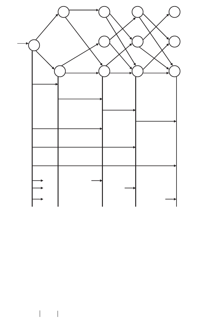
This is formally expressed as

p =·1, 0, 0Ò. Maximum and actual uncertainties

for some predictions are given in Figure 3.4. The diagram, which contains all

sequences of states with nonzero probabilities of length 4 or less, also shows

probabilities of individual states at each of the considered times. Each of the

arrows under the diagram indicates the time at which the prediction is made

and the time span of the prediction. Each of the ﬁrst four arrows is a predic-

tion about the next-time probability distributions made at different times.The

next three arrows indicate predictions made at time t about sequences of states

of lengths 2, 3, and 4. The last three arrows indicate predictions made at time

t about probability distributions at time t + 2, t + 3, and t + 4. The two numbers

on top of each arrow indicate the two uncertainties needed for calculating the

informativeness of the prediction, the maximum one and the actual one. Let

us follow in detail the calculation of some of these uncertainties.

Using Figure 3.4 as a guide, the next state prediction made at t + 2 is cal-

culated by the formula

tt++

=¥

ppM.

mpxx

()

px x Xp =

()

3.2. SHANNON MEASURE OF UNCERTAINTY FOR FINITE SETS 87

Substituting for

t+2

p and M, we obtain

Its uncertainty is measured by the conditional Shannon entropy

Sp x x ij S S

()

[]

=◊

()

+◊

()

+◊

()

018 00 0901 006 02 00 08

076 00 0604

0 866

, . .,.,. . .,.,.

. .,.,.

⺞

[]

018 006076

00 09 01

02 00 08

00 06 04

0 012 0 618 0 370

p .,.,.

...

.,.,. .

88 3. CLASSICAL PROBABILITY-BASED UNCERTAINTY THEORY

0.9

0.2

0.18

0.9

0.1

0.012 0.1236

0.2328

0.6436

0.9

0.1

0.618

0.2

0.8

0.370

0.6

0.4 0.4 0.4

0.1

0.6

0.8

0.06

0.2

0.8

0 .76

0.6

1.585

0.469

1.585

0.747

1.585

0.866

1.585

0.811

3.17

1.216

4.755

2.082

6.34

2.893

1.585

0.99

1.585

1.036

1.585

1.272

t t + 1 t + 2 t + 3 t + 4

Figure 3.4. Predictive uncertainties of the system deﬁned in Example 3.5.

which is calculated here by using Eq. (3.32). Its maximum counterpart, S

,is

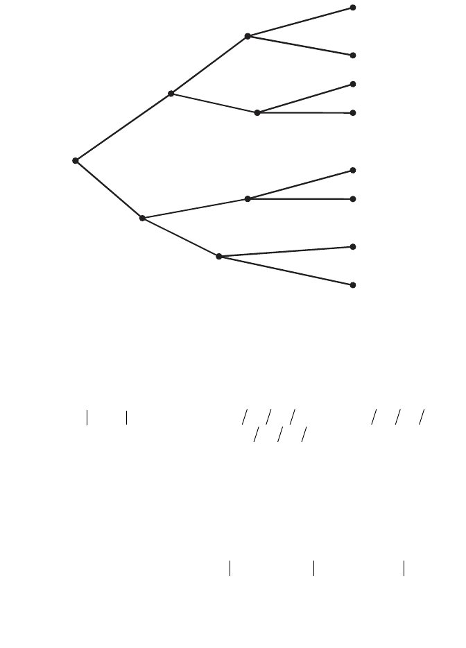
Now consider the prediction made at time t of sequences of states of length

3.There are, of course, 3

= 27 such sequences, but only 8 of them have nonzero

probabilities; these are shown in Figure 3.5. Probabilities of these sequences

are calculated by the formula

for all i, j, k Œ ⺞

. For example,

The amount of uncertainty in predicting at time t sequences of states at times

t + 1, t + 2, t + 3 is measured by the Shannon entropy for the probability dis-

tribution obtained for the sequences and shown in Figure 3.5. Its value is 2.082.

Since there are 27 possible sequences of states of length 3, the associated

maximum uncertainty is clearly equal to log

27 = 4.755.

px x x

tt t++ +

()

=¥¥¥=

1 0 9 0 8 0 6 0 432,, .....

px x x px pxx p x x px x

++ + + + + + +

()

12 3

21 3 2

,.,,.,,

.,,

log . .

Sp x x ij S S

()

[]

=◊

()

+◊

()

+◊

()

018 131313 006 131313

076 131313

3 1 585

⺞

3.2. SHANNON MEASURE OF UNCERTAINTY FOR FINITE SETS 89

: 0.162

: 0.018

: 0.432

: 0.288

: 0.012

: 0.048

: 0.024

: 0.016

0.9

0.8

0.2

0.9

0.1

0.6

0.4

0.2

0.8

0.6

0.4

0.1

0.6

Figure 3.5. Probabilities of sequences of states of length 3 in Example 3.5.

Predicting at time t sequences of states at times t + 1, t + 2, and t + 3 is, of

course, very different from predicting states at time t + 3. The latter prediction

is based on probabilities

for all i, k Œ⺞

. Since p(

) = 1 in our case, the only relevant probabilities are

The predictive uncertainty is thus equal to S(0.012, 0.618, 0.370) = 1.036, and

the maximum counterpart is equal to log

3 = 1.585.

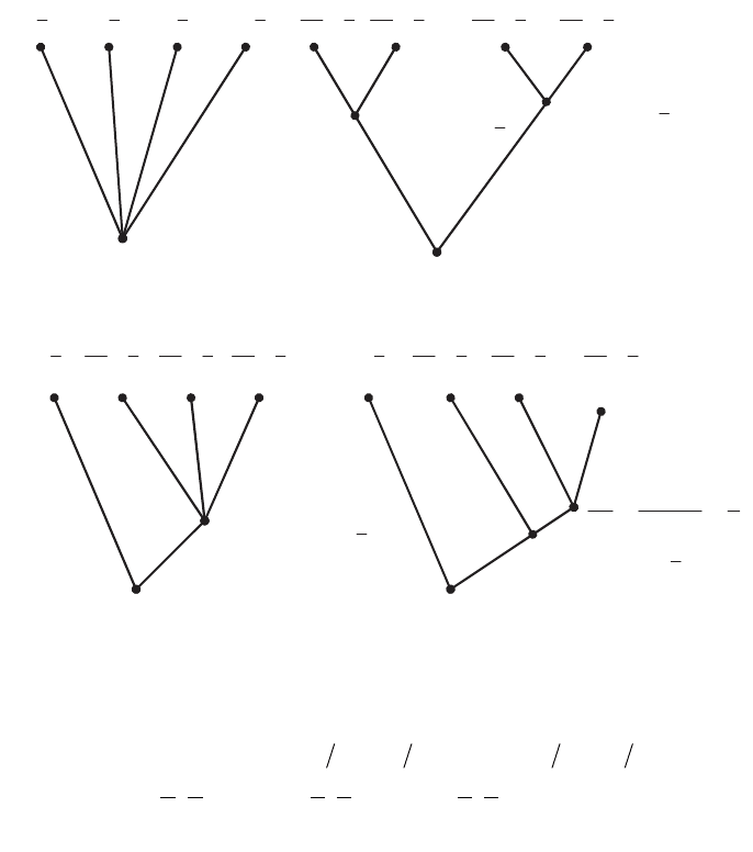
EXAMPLE 3.6. Let the set X = {x

, x

} with the probability distribution

be given where p

denotes the probability of x

for all i Œ ⺞

. Consider the

four branching schemes speciﬁed in Figure 3.6 for calculating the uncertainty

of this probability distribution. Employing the branching property of the

Shannon entropy, the resulting uncertainty should be the same regardless of

which of the branching schemes we use. Let us perform and compare the four

schemes of calculating the uncertainty.

Scheme I. According to this scheme, we calculate the uncertainty directly:

Scheme II

Scheme III

Sp Sp p p Sp p p p p p

AA A A A

()

+◊

()

+◊

=+=

1234

075

0 811 0 939 1 75

,,,

,. ,,

....

Sp Sp p p Sp p p p p Sp p p p

SSS

AB A A A B B B

()

+◊

()

+◊

()

+◊

=++=

,, ,

,. ,. ,

.....

12 34

075

025

0 811 0 689 0 25 1 75

()

=- - - ¥

=++ =

0 25 0 25 0 5 0 5 2 0 125 0 125

05 05 075 175

22 2

. log . . log . . log .

... ..

p == = = =ppp p

123 4

0 25 0 5 0 125 0 125., ., . , .

pxx

()

0 012

0 618

0 370

px p x x

()

◊

()

90 3. CLASSICAL PROBABILITY-BASED UNCERTAINTY THEORY

Scheme IV

These results thus demonstrate that the uncertainty can be calculated in terms

of any branching scheme. There are, of course, many additional branching

schemes in this example, each of which can be employed for calculating the

uncertainty and each of which must lead to the same result.

3.3. SHANNON-LIKE MEASURE OF UNCERTAINTY FOR

INFINITE SETS

One important aspect of the Shannon entropy remains to be discussed. This

aspect concerns its restriction to ﬁnite sets. Is this restriction necessary? It is

suggestive that the function

Sp Sp p p Sp p p p p Sp p p p

SSS

AA ABAB B B

()

+◊

()

+◊

()

+◊

=++=

12 34

075

025

0 811 0 689 0 25 1 75

,, ,

,. ,. ,

.....

3.3. SHANNON-LIKE MEASURE OF UNCERTAINTY FOR INFINITE SETS 91

( p)

Scheme I

( p

, p

)

Scheme II

( p

, p

)

Scheme III

( p

, p

, ( p

, p

))

Scheme IV

=+=

ppp

432

=++=

pppp

=+=

ppp

432

=++=

pppp

Figure 3.6. Application of the branching property of Shannon entropy.