Klir G.J. Uncertainity and Information. Foundations of Generalized Information Theory

Подождите немного. Документ загружается.

we need to recognize and work with the whole set of possible probability dis-

tributions, and not to choose only one of them, as required by probability

theory. This means, in turn, that we need to work with imprecise probabilities,

as shown in the rest of this section.

Sets of probability distribution functions deﬁned on some universal set X

are often referred to in the literature as credal sets on X. This shorter term is

convenient and it is occasionally used in this book.

4.3.1. Lower and Upper Probabilities

Let X denote a ﬁnite universal set of concern (a set of elementary events) and

let D denote a given set of probability distribution functions (a credal set), p,

on X.Then, the associated lower probability function,

, is deﬁned for all sets

A ŒP(X) by the formula

(4.11)

Similarly, the associated upper probability function,

, is deﬁned for all

A ŒP(X) by the formula

(4.12)

It follows directly from Eqs. (4.11) and (4.12) that lower and upper probabil-

ities are monotone measures.

Given a particular set A Œ P(X), let p

denote one of the probability distri-

bution functions in D for which the inﬁmum in Eq. (4.11) is obtained. Since

is required by probability theory for each set A Œ P(X), p

must also be a prob-

ability distribution function for which the supremum in Eq. (4.12) is obtained.

Hence, the equation

(4.13)

holds for all A ŒP(X). Due to this property, functions

and

are called

dual (or conjugate). One of them is sufﬁcient for capturing information in D;

the other one is uniquely determined by Eq. (4.13).

It follows directly from Eqs. (4.11) and (4.12) that

(4.14)

for all A ŒP(X) and, in addition,

mmAA

()

mmAA

()

–

˙˙

px px

xA xA

()

Œœ

ÂÂ

m Apx

()

sup .

m Apx

()

inf .

112 4. GENERALIZED MEASURES AND IMPRECISE PROBABILITIES

(4.15)

(4.16)

Moreover, any lower probability function is superadditive. That is,

(4.17)

for all A, B ŒP(X) such that A « B =∆. This follows form the fact that the

inﬁma for disjoint sets A and B may be obtained in Eq. (4.11) for distinct prob-

ability distribution functions in D,but the inﬁmum for A » B must be obtained

for a single probability distribution function in D. By the same argument

applied to the suprema for A, B, and A » B in Eq. (4.12), it follows that the

upper probability function is subadditive. That is,

(4.18)

for all A, B ŒP(X ).

Lower probabilities also satisfy the inequality

(4.19)

This can be shown by using Eqs. (4.16) and (4.17), and the associativity of the

operation of set union:

In a similar way, it can be shown that

(4.20)

Due to the inequality (4.14), the lower and upper probabilities form for

each set A Œ P(X) a closed interval

of possible probabilities of that set. When

(A) =

(A) for all A ŒP(X),

classical (precise) probabilities are obtained. It is important to realize that a

lower probability function (or,alternatively, an upper probability function) can

be derived from more than one set of probability distribution functions on a

given set X. This possibility is illustrated by the following example.

mmAA

() ()

[]

m x

{}()

≥

1 =

()

{}

≥

{}()

DD D

mm mXx x

m x

{}()

DDD

mmmAB A B»

()

DDD

mmmAB A B»

()

≥

()

mmXX

()

= 1.

mm∆

()

=∆

()

= 0,

4.3. IMPRECISE PROBABILITIES: GENERAL PRINCIPLES 113

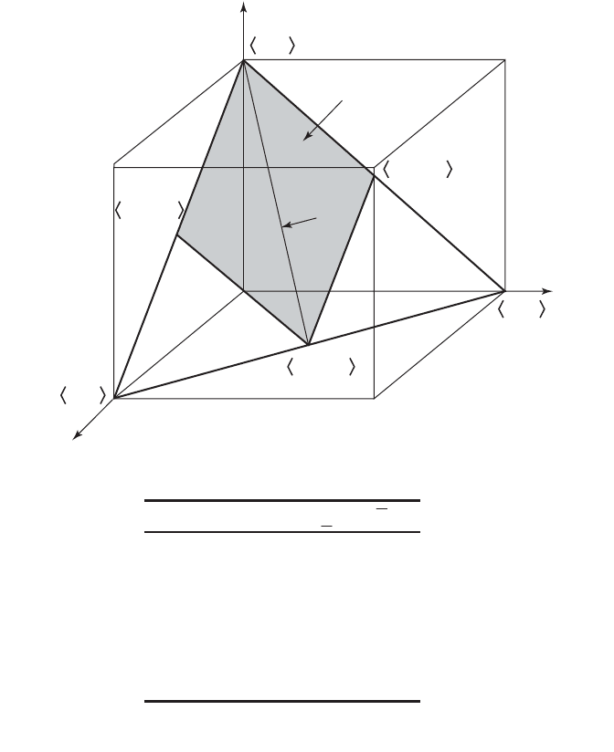
EXAMPLE 4.4. Consider X = {x

, x

} and the following two sets of prob-

ability distributions on X:

A geometrical interpretation of these sets is shown in Figure 4.3a. It is easy to

see that applying Eqs. (4.11) and (4.12) to these sets results in the same lower

and upper probability functions given in Figure 4.3b. Moreover,any set D such

that D

 D  D

is also associated with these functions.

Associated with any given lower probability function on P(X ) is the

unique set,

D, of all probability distribution functions p on X that are

consistent with (or dominate ). That is,

(4.21)

Clearly,

D is the largest among those sets of probability distribution

functions on X that are associated with . Given the lower probability func-

tion in Example 4.4, the unique set

D deﬁned by Eq. (4.21) is clearly the

set D

Alternatively, the set of all probability distributions p on X that are con-

sistent with a given upper probability function m

on P(X) (or are dominated

by m

) is deﬁned as follows:

(4.22)

However,

D =

D due to the duality of and m

. Introducing the symbol

for any dual pair of lower and upper probability functions, the symbols

D and

D may conveniently be replaced with one common symbol

It is important to realize that

D is always a closed convex set of probabil-

ity distribution functions on X. It is the intersection of the closed convex

sets of probability distribution functions characterized by the individual

inequalities in Eqs. (4.21) or (4.22).When m is derived by Eqs. (4.11) and (4.12)

from a given set D that is not convex, then D is not necessarily contained in

All lower probability functions are superadditive and so are all Choquet

capacities of any order k ≥ 2. These two classes of functions are thus compat-

ible.This means that special types of Choquet capacities (of the various orders

k ≥ 2) represent in a natural way special types of lower probability functions.

m = mm,

mDP=

()

≥

()

pA px A X

for all .

mDP=

()

pA px A X

for all .

1 123 1 2 3

2 123 1 2

12 005

1005

()() () ()

()

=- Œ

[]

{}

()() () ()

()

{

()

=-- Œ

[]

px px px px px a px a a

px px px px a px b

px a ba b

,, , , ,.,

,, , ,

,,.,ŒŒ

[]

}

005,. .

114 4. GENERALIZED MEASURES AND IMPRECISE PROBABILITIES

That is, Choquet capacities of each order form a basis for formalizing a par-

ticular theory of imprecise probabilities.

4.3.2. Alternating Choquet Capacities

Due to the duality of lower and upper probabilities expressed by Eq. (4.13),

each theory of imprecise probabilities may also be formalized in terms of the

upper probabilities. In that case, Choquet capacities that are dual to those pre-

4.3. IMPRECISE PROBABILITIES: GENERAL PRINCIPLES 115

x (A)

(A)

0 0 0 0.0 0.0

1 0 0 0.0 0.5

0 1 0 0.0 0.5

0 0 1 0.0 1.0

1 1 0 0.0 1.0

1 0 1 0.5 1.0

0 1 1 0.5 1.0

1 1 1 1.0 1.0

(b)

(a)

p(x

)

p(x

)

p(x

)

0, 1, 0

0.5, 0.5, 0

0, 0.5, 0.5

0.5, 0, 0.5

1, 0, 0

0, 0, 1

Figure 4.3. Illustration to Example 4.4.

viously introduced must be used. They are called alternating Choquet capaci-

ties of order k (or k-alternating Choquet capacities) and are deﬁned for all fam-

ilies of k subsets of X (k ≥ 2) by the inequalities

(4.23)

Moreover, alternating Choquet capacities of order • (or •-alternating) are

deﬁned by the inequalities

(4.24)

for every k ≥ 2 and every family of k subsets of X.

4.3.3. Interaction Representation

Given a ﬁnite universal set X = {x

| i Œ⺞

}, let X

denote the set of all n! per-

mutations of X. Denoting for convenience, the set of all permutations of ⺞

by P

, we have

For each p ŒP

and each k Œ⺞

, let

and let A

p,0

=∆for any p ŒP

by convention. Clearly, the sequence of sets A

p,k

for all k Œ⺞

0,n

is one particular maximal chain of nested subsets of X in the

Boolean lattice ·P(X), Ò. This chain is uniquely characterized by the chosen

permutation p. Given a regular monotone measure m on P(X ), a sequence of

values m(A

p,k

) for k Œ⺞

0,n

is associated with subsets in the chain. Clearly, m(A

p,0

)

= 0, m(A

p,n

) = 1,

for all k Œ⺞

, and

Hence, probability distribution functions,

p, deﬁned for each particular

p ŒP

and all k Œ⺞

by the formula

()

[]

kk,,

()

[]

-1

Axx x

kkppp p,

, ,..., ,=

{}

() () ()

Xxi

inn

,.== Œ Œ

{}

()

p⺞ P

mmm

AA A A AA

AA A

«««

()

-»

()

»»»

()

ÂÂ

... ...

...

mmAA

π∆

£-

()

116 4. GENERALIZED MEASURES AND IMPRECISE PROBABILITIES

(4.25)

are induced by m in the Boolean lattice ·P(X), Ò. Clearly, functions deﬁned

for different permutations are not necessarily distinct. Let

B denote the set

of all distinct probability functions deﬁned by Eq. (4.25). Then, clearly, 1 £|

£ n!.

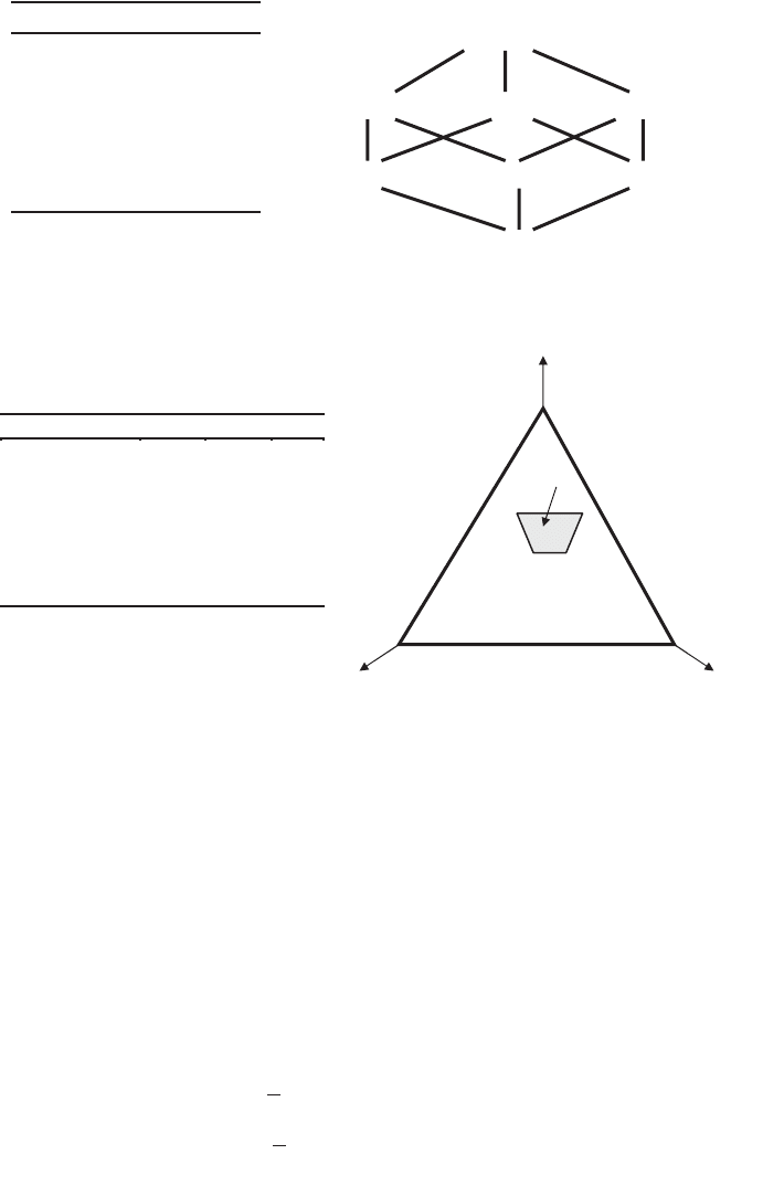
EXAMPLE 4.5. Two distinct monotone measures, m

and m

, are deﬁned in

Figures 4.4a and 4.5a. In Figures 4.4b and 4.5b, respectively, these measures

are expressed in terms of the Hasse diagrams of the underlying Boolean

lattice. Measure m

is additive and, hence, it is completely characterized by a

single probability distribution function p whose values are equal to the values

of m

for singletons. It can be easily veriﬁed that functions

p for all p ŒP

are equal to p. Measure m

is a Choquet capacity of order 2. Functions

p for

all p ŒP

are shown in Figure 4.5c. Clearly,

B consists in this case of four

probability distributions, p

, p

, as is obvious from Figure 4.5c.

The explained representation of a given monotone measure m by the asso-

ciated set

B of probability distribution functions is usually called an interac-

tion representation in the literature. The term “interaction” refers to the

capability of monotone measures to express positive or negative interactions

among disjoint sets with respect to the measured property. It turns out that

the interactions intrinsic to a monotone measure m are more explicitly

expressed by the associated set

The following are some basic properties for the interaction representation

of monotone measures that pertain to imprecise probabilities (see Note 4.4):

ppp

mmpx A A

kkk

()

,,1

4.3. IMPRECISE PROBABILITIES: GENERAL PRINCIPLES 117

x )(

0 0 0 0.0

1 0 0 0.5

0 1 0 0.3

0 0 1 0.2

1 1 0 0.8

1 0 1 0.7

0 1 1 0.5

1 1 1 1.0

}: 1.0

}: 0.8 {x

}: 0.7 {x

}: 0.5

}: 0.5 { x

}: 0.3 {x

}: 0.2

∆

: 0.0

(a) (b)

Figure 4.4. Interaction representation of additive measure m

(Example 4.5).

(i1) For any pair of dual monotone measures, m =· , m

Ò,

B =

B, but the

same probability functions in

B and

B are obtained for different per-

mutations.

(i2) A monotone measure m is additive iff |

B|=1.

(i3) Let m =· , m

Ò be a pair of dual monotone measures, so that

B =

B. Then, is a Choquet capacity of order 2 (and m

is the associated

alternating capacity of order 2) iff

(4.26)

(4.27)

m Apx

()

max

m Apx

()

min ,

118 4. GENERALIZED MEASURES AND IMPRECISE PROBABILITIES

) p

)

1, 2, 3

1, 3, 2

0.2

0.3

0.5

2, 1, 3

2, 3, 1

0.4

0.1

0.5

3, 1, 2

0.3 0.3 0.4

3, 2, 1

0.4 0.2 0.4

(A)

0 0 0 0.0

1 0 0 0.2

0 1 0 0.1

0 0 1 0.4

1 1 0 0.5

1 0 1 0.7

0 1 1 0.6

1 1 1 1.0

, x

}: 1.0

, x

}: 0.5 {x

, x

}: 0.7 {x

, x

}: 0.6

}: 0.2 {x

}: 0.1 {x

}: 0.4

∆

: 0.0

(a) (b)

(c)

p(x

)

0, 0, 1

p(x

)

1, 0, 0

p(x

)

0, 1, 0

(d )

Figure 4.5. Interaction representation of 2-monotone measure (Example 4.5).

for all A Œ P(X).When and m

are more general monotone measures,

Eqs. (4.26) and (4.27) are not applicable.In that case, and m

are deter-

mined from

B if the permutations corresponding to each probability

distribution function

B are known.

(i4) A given monotone measure m is a Choquet capacity of order 2 iff

B 

(i5) If a given monotone measure m is a Choquet capacity of order 2, then

B is the set of extreme points of

D, which is commonly referred to

as the proﬁle of

Property (i5) is particularly important. It allows us to determine

D directly

from the interaction representation

B provided that m is a Choquet capacity

of order 2.

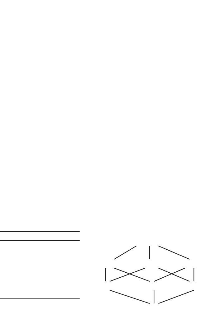
EXAMPLE 4.6. Consider the lower and upper probability functions and m

deﬁned in Figure 4.3b. Hasse diagrams of the Boolean lattice with values

(A) and m

(A) are shown in Figure 4.6a and 4.6b, respectively. Probability dis-

tribution functions

p and

p for all permutations p ŒP

are shown in Figure

4.6c and 4.6d, respectively. We can see that

B =

B is the set of the

extreme points of

D, which are shown in Figure 4.3a.

EXAMPLE 4.7. The lower probability function m

deﬁned in Figrue 4.5a is a

Choquet capacity of order 2.According to property (i5) of the interaction rep-

resentation,

B = {p

, p

} (given in Figure 4.5c) is the set of extreme

points of

D. Hence,

D is characterized by the linear combination of these

points. Locations of the extreme points in the probabilistic simplex and the set

of all points in

D are shown in Figure 4.5d.

4.3.4. Möbius Representation

When the Möbius transform in Eq. (4.8) is applied to lower and upper prob-

ability functions, and m

, distinct functions, m

–

and m

, are obtained respec-

tively. By applying the inverse transform in Eq. (4.9) to m

–

and m

, we obtain

–

and m

, respectively. Since the functions and m

are dual, the corresponding

functions m

–

and m

are dual as well. It is established that the duality of the

latter functions is expressed for all A ŒP(X) by the equation

(4.28)

For more information, see Note 4.4.

EXAMPLE 4.8. Lower and upper probability functions, and m

, and their

Möbius representations, m

–

and m

, are given in Table 4.3. Since functions and

mA mB

BB A

()

() ()



4.3. IMPRECISE PROBABILITIES: GENERAL PRINCIPLES 119

120 4. GENERALIZED MEASURES AND IMPRECISE PROBABILITIES

}: 1.0

}: 1.0 {x

}: 1.0

{ x

}: 0.5 { x

}: 0.5 {x

}: 1.0

∆: 0.0

(b)

}: 1.0

}: 0.0 {x

}: 0.5 {x

}: 0.5

{ x

}: 0.0 { x

}: 0.0 {x

}: 0.0

∆: 0.0

(a)

) p

)

·1, 2, 3Ò

·2, 1, 3Ò

0.0

1.0

·1, 3, 2Ò

0.0 0.5 0.5 p

·2, 3, 1Ò

0.5 0.0 0.5 p

·3, 1, 2Ò

·3, 2, 1Ò

0.5

0.0

) p

)

·1, 2, 3Ò

·2, 1, 3Ò

0.5

0.0

·1, 3, 2Ò

0.5 0.0 0.5 p

·2, 3, 1Ò

0.0 0.5 0.5 p

·3, 1, 2Ò

·3, 2, 1Ò

0.0

1.0

(c)

(d)

Figure 4.6. Illustration to Example 4.6.

Table 4.3. Duality of Möbius Representations of Lower and Upper Probability

Functions (Example 4.8)

(A) m

(A)

A: 0 0 0 0.0 0.0 0.0 0.0

1 0 0 0.1 0.1 0.4 0.4

0 1 0 0.3 0.3 0.7 0.7

0 0 1 0.2 0.2 0.5 0.5

1 1 0 0.5 0.1 0.8 -0.3

1 0 1 0.3 0.0 0.7 -0.2

0 1 1 0.6 0.1 0.9 -0.3

1 1 1 1.0 0.2 1.0 0.2

are dual, m

–

and m

are dual as well.This means that they uniquely determine

each other via Eq. (4.28). For example,

4.3.5. Joint and Marginal Imprecise Probabilities

Let D,,m

and m denote the four basic representations of joint imprecise

probabilities on a Cartesian product X ¥ Y, and let D

, D

, m

and m

denote their marginal counterparts. For each of the four basic repre-

sentations of the joint imprecise probabilities, its marginal counterparts are

determined by appropriate rules of projection that are deﬁned as follows.

•

Marginal sets of probability distributions:

(4.29)

(4.30)

•

Marginal lower probabilities:

(4.31)

(4.32)

•

Marginal upper probabilities:

(4.33)

(4.34)

•

Marginal Möbius functions:

(4.35)

mA mR A X

RA R

()

for all P ,

BXB BY

()

=¥

()

for all P .

AAY AX

()

=¥

()

for all P ,

BXB BY

()

=¥

()

for all P .

AAY AX

()

=¥

()

for all P ,

YYY

ppy pxy p=

()

,. for some

XXX

ppx pxy p=

()

,, for some

mxx mxx mxxx

mx mx mxx mx x mxx x

12 12 123

3 3 13 23 123

01 02 03

02 00 0

,,,,

.. .,

,,,,

...

{}()

[]

=- +

[]

{}()

{}(

)

=++1102 05

01 02 03

23 23 123

{}()

[]

=- +

[]

..,

,,,,

.. ..

mxx mxx mxxx

4.3. IMPRECISE PROBABILITIES: GENERAL PRINCIPLES 121