Klir G.J. Uncertainity and Information. Foundations of Generalized Information Theory

Подождите немного. Документ загружается.

(4.36)

where

It is well established that marginal lower and upper probability functions

calculated by these formulas are measures of the same type as the given joint

lower and upper probability functions.

4.3.6. Conditional Imprecise Probabilities

Given a lower probability function or an upper probability function m

P(X), a natural way of deﬁning conditional lower probabilities (A | B) for

any subsets A, B of X is to employ the associated convex set of probability

distribution functions D (deﬁned by Eq. (4.21) or Eq. (4.22), respectively). For

each p Œ D, the conditional probability is deﬁned in the classical way,

and Eqs. (4.11) and (4.12) are modiﬁed for the conditional probabilities to

calculate the lower and upper conditional probabilities. That is,

(4.37)

(4.38)

for all A, B Œ P(X).

Consider now joint lower and upper probability functions and m

on P(X

¥ Y ) and the associated set D of joint probability distribution functions p that

dominate and are dominated by m

. Then, for all A ŒX, B ŒY and p ŒD,

Pro A B

Pro X B

px y

xy A B

xy X B

()

Œ¥

m AB

xA B

()

Œ«

sup ,

m AB

xA B

()

Œ«

inf ,

Pro A B

Pro B

()

RyYxyR xX

=Œ Œ Œ

{}

,. for some

RxXxyR yY

=Œ Œ Œ

{}

,, for some

mB mR B Y

RB R

()

for all P ,

122 4. GENERALIZED MEASURES AND IMPRECISE PROBABILITIES

and (A | B) or m

(A | B) are obtained, respectively, by taking the inﬁmum or

supremum of Pro(A | B) for all p ŒD. Similarly,

and (B | A) or m

(B | A) are obtained, respectively, by taking the inﬁmum or

supremum of Pro(B | A).

4.3.7. Noninteraction of Imprecise Probabilities

It remains to address the following question: Given marginal imprecise prob-

abilities on X and Y, how to deﬁne the associated joint imprecise probabili-

ties under the assumption that the marginal ones are noninteractive? The

answer depends somewhat on the type of monotone measures by which the

marginal imprecise probabilities are formalized, as is discussed in Chapters 5

and 8. However, when operating at the general level of Choquet capacities of

order 2, the question is adequately answered via the convex sets of probabil-

ities distributions associated with the given marginal lower and upper proba-

bilities as follows:

(a) Given marginal lower and upper probability functions, m

=·

, m

Ò and

=·

, m

Ò, on P(X) and P(Y), respectively, determine the associated

convex sets of marginal probability distributions, D

and D

, on X and

(b) Assuming that m

and m

are noninteractive, apply the notion of non-

interaction in classical probability theory, expressed by Eq. (3.7), to

probability distributions in set D

and D

to deﬁne a unique set of

joint probability distributions, D, on set X ¥ Y.

probability functions m =·

Ò. These are, by deﬁnition, the unique

joint lower and upper probability functions that correspond to non-

interactive marginal lower and upper probability functions m

and m

It is known (see Note 4.5) that the following properties hold under this

deﬁnition for all A ŒP(X) and all B ŒP(Y):

(4.39)

(4.40)

(4.41)

mmmmmAY X B A B A B

XYXY

()

»¥

()

[]

()

◊

()

mmmAB A B

()

◊

()

mmmAB A B

()

◊

()

Pro B A

Pro A B

Pro A Y

px y

xy A B

xy A Y

()

Œ¥

4.3. IMPRECISE PROBABILITIES: GENERAL PRINCIPLES 123

(4.42)

Moreover, it is guaranteed that the marginal measures of m =· , m

Ò are again

the given marginal measures m

=·

, m

Ò and m

=·

, m

Ò.

EXAMPLE 4.9. Consider the marginal lower and upper probability functions

=·

, m

Ò and m

=·

, m

Ò on sets X = {x

, x

} and Y = {y

, y

}, respectively,

which are given in Table 4.4a. Assuming that these marginal probability func-

tions are noninteractive, the corresponding joint lower and upper probabili-

ties m =·, m

Ò are uniquely determined by the introduced deﬁnition of

noninteraction. One way to compute them is to directly follow the deﬁnition

of noninteraction. Another, more convenient way is to use Eqs. (4.39)–(4.42)

for all subsets of X ¥ Y for which the equations are applicable and use the

direct method only for the remaining subsets.

Following the deﬁnition of noninteraction, we need to determine ﬁrst the

convex sets D

and D

of marginal probability distributions. From Table 4.4a,

Hence, D

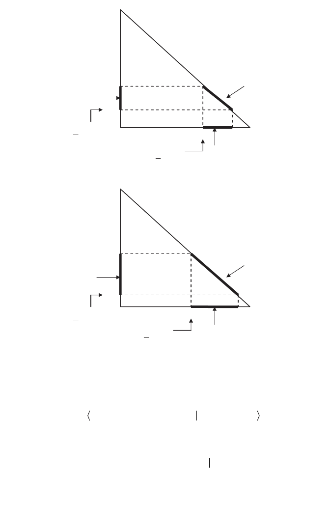
is the convex combination of the extreme distributions,

that dominate the lower probabilities (Figure 4.7a) or, alternatively, are dom-

inated by the upper probabilities (Figure 4.7c). That is,

and

Similarly,

YYYY

05 091 01

09 04 01

05 011 01

01 04 01

()

Œ+-

()

[]

{}

=- Œ

[]

{}

()

Œ+-

()

[]

{}

=+ Œ

[]

{}

.. ,

.. ,,

lll

XXXX

=- + Œ

[]

{}

08 02 02 02 01..,.. ,.lll

XXXX

06 081 01

08 02 0 1

04 021 01

02 02 0 1

()

Œ+-

()

[]

{}

=- Œ

[]

{}

()

Œ+-

()

[]

{}

=+ Œ

[]

{}

.. ,

lll

px px px px

XX XX12 12

06 04 08 02

()

=., . ., . ,and

px px

py py

0608 02 04

0509 0105

()

[]

()

[]

()

[]

()

[]

., . , ., .

., . , ., . .

mmmmmAY X B A B A B

XYXY

()

»¥

()

[]

()

◊

()

124 4. GENERALIZED MEASURES AND IMPRECISE PROBABILITIES

(A) m

(A)

A: 0 0 0.0 0.0

1 0 0.6 0.8

0 1 0.2 0.4

1 1 1.0 1.0

(B) m

(B)

B: 0 0 0.0 0.0

1 0 0.5 0.9

0 1 0.1 0.5

1 1 1.0 1.0

(a)

and

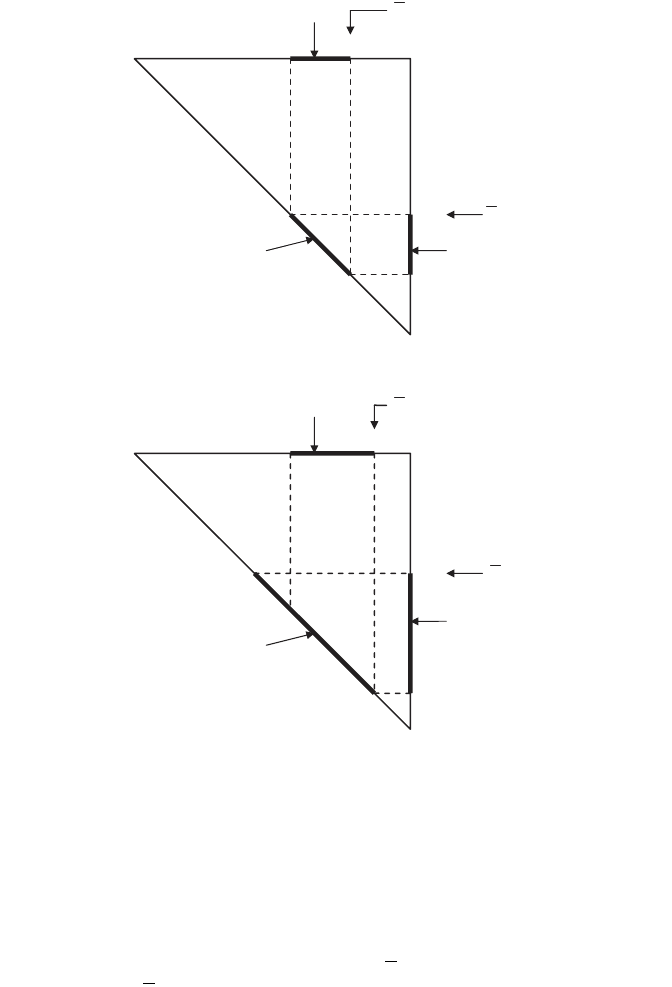
as can be derived with the help of Figure 4.7b (or alternatively, Figure 4.7d).

Values of l

and l

are independent of each other.

Now applying the deﬁnition of noninteraction, we determine the set D of

joint probability distributions p by taking pairwise products of components of

the marginal probability distributions. That is,

YYYX

=- + Œ

[]

{}

09 04 01 04 01..,.. ,,lll

4.3. IMPRECISE PROBABILITIES: GENERAL PRINCIPLES 125

Table 4.4. Joint Lower and Upper Probability Functions Based on Noninteractive

Marginal Lower and Upper Probability Functions (Example 4.9)

C: 0 0 0 0 0.00 0.00 0.00

1 0 0 0 0.30 0.72 0.30

0 1 0 0 0.06 0.40 0.06

0 0 1 0 0.10 0.36 0.10

0 0 0 1 0.02 0.20 0.02

1 1 0 0 0.60 0.80 0.24

1 0 1 0 0.50 0.90 0.10

1 0 0 1 0.50 0.74 0.18

0 1 1 0 0.26 0.50 0.10

0 1 0 1 0.10 0.50 0.02

0 0 1 1 0.20 0.40 0.08

1 1 1 0 0.80 0.98 -0.10

1 1 0 1 0.64 0.90 -0.18

1 0 1 1 0.60 0.94 -0.18

0 1 1 1 0.28 0.70 -0.10

1 1 1 1 1.00 1.00 0.36

(b)

For example,

Clearly, the minimum p(x

, y

) is 0.3, and it is obtained for l

= l

= 1; the

maximum is 0.72, and it is obtained for l

= l

= 0. Hence,

px y

03072,.,.,

()

[]

px y

XYXY11

08 02 09 04 01,.... ,,.

()

Œ-

()

[]

{}

llll

D =

()

◊

()

ŒŒ

{}

px y p x p y x X y Y

ij X Yj i j

,,.

126 4. GENERALIZED MEASURES AND IMPRECISE PROBABILITIES

(a)

(b)

})({

0.9, 0.1

0.5, 0.5

})({

)

0.1

0.5

0.90.5

)

})({

0.8, 0.2

0.6, 0.4

})({

)

0.2

0.4

0.80.6

)

Figure 4.7. Illustration to Example 4.9. (a) D

via lower probability m

. (b) D

via lower

probability m

and, consequently,

Similarly,we can calculate the ranges of joint probabilities p(x

, y

) for the other

pairs of x

ŒX and y

ŒY whose minima and maxima are the joint lower and

upper probabilities of singleton sets, which are given in Table 4.4b:

mmxy xy

11 11

03 072,. ,..

{}()

=and

4.3. IMPRECISE PROBABILITIES: GENERAL PRINCIPLES 127

0.4

0.8

0.2

·0.6, 0.4Ò

·0.8, 0.2Ò

0.6

(

)

})({

(

)

})({

0.5

0.9

0.1

·0.5, 0.5Ò

·0.9, 0.1Ò

0.5

(

)

})({

(

)

})({

(c)

(d )

Figure 4.7. (c) D

via upper probability m

. (d ) D

via upper probability m

We can also calculate ranges of joint probability measures, Pro, for the other

subsets of X ¥ Y by adding the respective products of marginal probability.

The minima and maxima of these ranges are, respectively, the lower and upper

probabilities of these subsets (shown in Table 4.4b). For example,

Using Eqs. (4.39)–(4.42), the joint lower and upper probabilities can be cal-

culated more conveniently for all subsets of X ¥ Y except the subsets {·x

, y

Ò,

·x

, y

Ò}, and {·x

, y

Ò, ·x

, y

Ò}. For example,

mmm

xy x y

11 1 1

06 05 03

08 09 072

.. .,

{}()

◊

{}()

=◊=

{}()

◊

{}()

=◊=

Pro x y x y x y

XYXY

11 1 2 21

08 02 09 04

08 02 01 04

02 02 09 04 01

0 98 0 02 0

,,,,, . . . .

.. ..

.. .. , ,

{}()

Œ-

()

(){

()

[]

}

=- -

llll

l ..

.,,

.,. .

008 01

080 098

ll l l

XY X Y

{

-Œ

[]

}

[]

Pro x y x y

XYXY

XYXYXY

11 22

08 02 09 04

02 02 01 04 01

074 016 024 016 01

050

,,, . . . .

.. .. , ,

.. . . , ,

{}

()

Œ-

()

{

()

[]

}

=- - + Œ

[]

{}

llll

llllll

,, . .074

[]

Pro x y x y

XYXY

XY XYXY

12 21

08 02 01 04

02 02 09 04 01

026 016 024 016 01

026

,,, . . . .

.. .. , ,

.. . . , ,

{}

()

Œ-

()

{

()

[]

}

=+ + - Œ

[]

{}

llll

llllll

,, . .050

[]

Pro x y x y

XYXY

11 1 2

08 02 09 04

08 02 01 04 01

08 02 0 1

0608

,,, . . . .

.. .. , ,

.. ,

., . .

{}()

Œ-

()

(){

()

[]

}

=- Œ

[]

{}

[]

llll

px y

XYXY

08 02 01 04 01

006040

02 02 09 04 0 1

01036

,.... ,,

.,. ,

,.... ,,

., . ,

()

Œ-

()

[]

{}

[]

()

Œ+

()

[]

{}

[]

(

llll

))

Œ+

()

[]

{}

[]

02 02 01 04 01

002 020

.. .. , ,

.,. .

llll

XYXY

128 4. GENERALIZED MEASURES AND IMPRECISE PROBABILITIES

4.4. ARGUMENTS FOR IMPRECISE PROBABILITIES

The need for enlarging the framework of classical probability theory by allow-

ing imprecision in probabilities has been discussed quite extensively in the

literature, and many arguments for imprecise probabilities have been put

forward. The following are some of the most common of these arguments.

1. Situations in which given information implies a set of probability distri-

butions on a given set X are quite common. One type of such situations is illus-

trated by Example 4.3. All these situations can be properly formalized by

imprecise probabilities, as is shown in Section 4.3, but not by classical, precise

probabilities. Choosing any particular probability distribution from the given

set, as is required by classical probability theory, is utterly arbitrary. Regard-

less how this choice is justiﬁed within classical probability theory, it is not sup-

ported by available information. The extreme case is reached in a situation of

total ignorance—a situation in which no information about probability distri-

butions is available. This situation, in which all probability distributions on X

are possible, is properly formalized by special lower and upper probability

functions that are deﬁned for all A ŒP(X) by the formulas

(4.43)

(4.44)

These lower and upper probabilities deﬁne, in turn, the following ranges of

probabilities, Pro, that are maximally imprecise:

m A

()

=∆

π∆

when

when .

m A

()

when

when .

mmmm

xy xy x y x Y X y

xyxy

xy xy x y

XYXY

11 1 2 21 1 1

11 11

11 1 2 2

06 05 06 05 08

,,,,,

.....,

,,,,,

{}()

{}

()

»¥

{}()

[]

{}()

◊

{}()

=+-◊=

111 1

11 11

08 09 08 09 098

{}()

{}

()

»¥

{}()

[]

{}()

◊

{}()

=+-◊=

mmmm

xY Xy

xyxy

XYXY

......

mmm

xy xy x Y

11 12 1

06 1 06

08 1 08

,,,

..,

,,,

..,

{}

()

{}

()

◊

()

=◊=

{}

()

{}

()

◊

()

=◊=

4.4. ARGUMENTS FOR IMPRECISE PROBABILITIES 129

and, of course, Pro(∆) = 0 and Pro(X) = 1. These maximally imprecise prob-

abilities are usually called vacuous probabilities. It is obvious that they are

associated with the set of all probability distributions on X.

2. Imprecision of probabilities is needed to reﬂect the amount of statisti-

cal information on which they are based. The precision should increase with

amount of statistical information. Imprecise probabilities allow us to utilize

this sensible principle methodologically. As a simple example, let X denote a

ﬁnite set of states of a variable and let the variable be observed at discrete

times. Assume that in a sequence of N observations of the variable, each state

x ŒX was observed n(x)-times.According to classical probability theory, prob-

abilities of individual states, p(x), are estimated by the ratios n(x)/N for all

x ŒX.While these estimates are usually acceptable when N is sufﬁciently large

relative to the number of all possible states, they are questionable when N is

small. An alternative is to estimate lower and upper probabilities, (x) and

(x), in such a way that we start with the maximum imprecision ( (x) = 0 and

(x) = 1 for all x Œ X) when N = 0 (total ignorance) and deﬁne the impreci-

sion (expressed by the differences (x) - m

(x)) by a function that is monot-

one decreasing with N. This can be done, for example, by using for each

x Œ X the functions (estimators)

(4.45)

(4.46)

where c ≥ 1 is a coefﬁcient that expresses how quickly the imprecision in esti-

mated probabilities decreases with the amount of statistical information,

which is expressed by the value of N. The chosen value of c expresses the

caution in estimating the probabilities.The larger the value, the more cautious

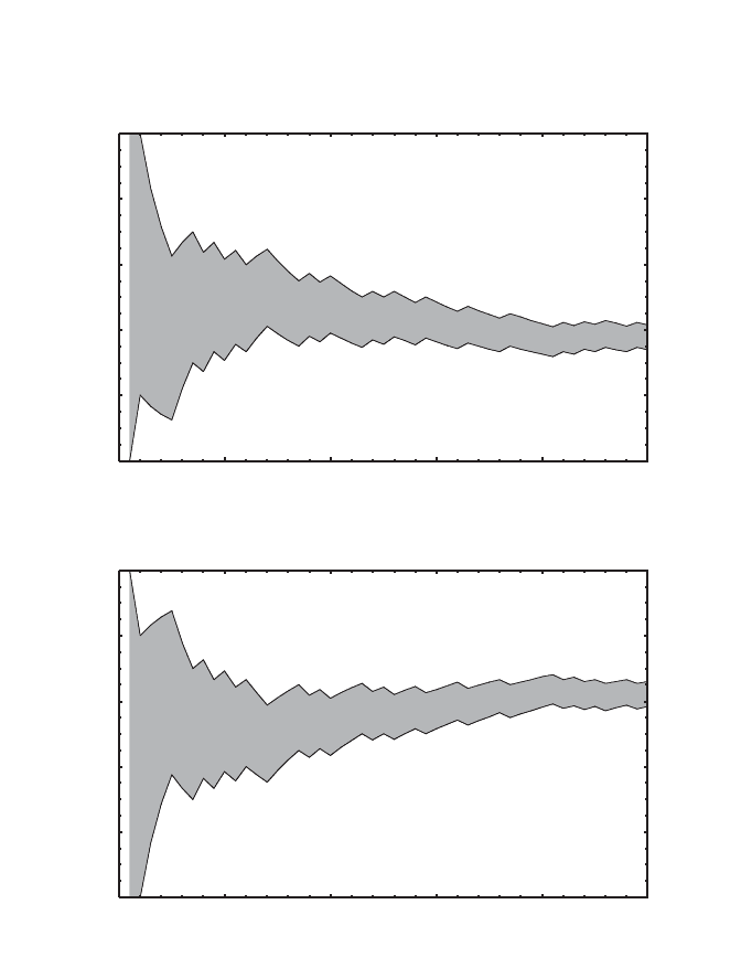
the estimators are. As a simple example, let X = {0, 1} be a set of states of a

single variable n, whose observations, n(t), at discrete times t Œ ⺞

are given

in Figure 4.8a. These observations were actually randomly generated with

probabilities p(0) = 0.39 and p(1) = 0.61. Figure 4.8b shows lower and upper

probabilities of x = 0 estimated for each N Œ ⺞

by Eqs. (4.45) and (4.46),

respectively, with c = 4. Figure 4.8c shows the same for x = 1.

3. Classical probability theory requires that Pro(A) + Pro(A

) = 1. This

means, for example, that a little evidence supporting A implies a large amount

of evidence supporting A

. However,in many real-life situations, we have a little

evidence supporting A and a little evidence supporting A

as well. Suppose, for

m x

nx c

()

m x

()

Pro A A X X

()

[]

()

-∆

{}

01,,,for all P

130 4. GENERALIZED MEASURES AND IMPRECISE PROBABILITIES

4.4. ARGUMENTS FOR IMPRECISE PROBABILITIES 131

example, that an old painting was discovered that somewhat resembles paint-

ings of Raphael. Such a discovery is likely to generate various questions

regarding the status of the painting. The most obvious questions are:

(a) Is the discovered painting a genuine painting by Raphael?

(b) It the discovered painting a counterfeit?

v (t) = 0111001010100111010111010

1101110111011110101011011

(a)

10 20 30 40 50

0.8

10 20 30 40 50

0.2

0.4

0.6

(b)

10 20 30 40 5010 20 30 40 50

0.2

0.4

0.6

0.8

(c)

Figure 4.8. Example of the decrease of imprecision in estimated probabilities with the

amount of statistical information.