Jean-Laurent Mallet. Geomodeling
Подождите немного. Документ загружается.

488
CHAPTER
9.
STOCHASTIC MODELING
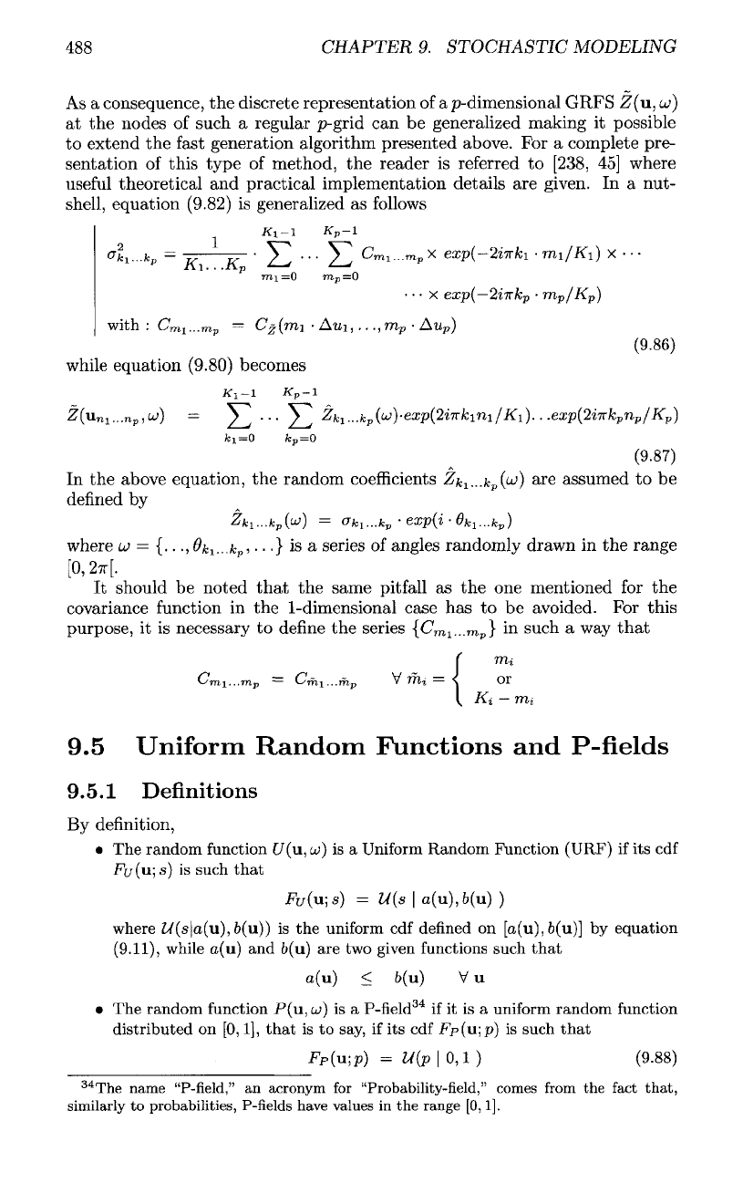
As
a
consequence,
the
discrete representation
of a
p-dimensional
GRFS
Z(u,
u)
at the
nodes
of
such
a
regular
p-grid
can be
generalized making
it
possible
to
extend
the
fast
generation algorithm presented above.
For a
complete pre-
sentation
of
this type
of
method,
the
reader
is
referred
to
[238,
45]
where
useful
theoretical
and
practical implementation details
are
given.
In a
nut-
shell,
equation
(9.82)
is
generalized
as
follows
while
equation (9.80) becomes
In the
above equation,
the
random
coefficients
^/
Cl
...fc
p
(^')
are
assumed
to be
defined
by
where
u
=
{...,
&k
v
...k
p
,
• • •} is a
series
of
angles
randomly drawn
in the
range
[0,27T[.
It
should
be
noted
that
the
same pitfall
as the one
mentioned
for the
covariance
function
in the
1-dimensional
case
has to be
avoided.
For
this
purpose,
it is
necessary
to
define
the
series
{C
mi
...
TOp
}
in
such
a way
that
9.5
Uniform
Random
Functions
and
P-fields
9.5.1
Definitions
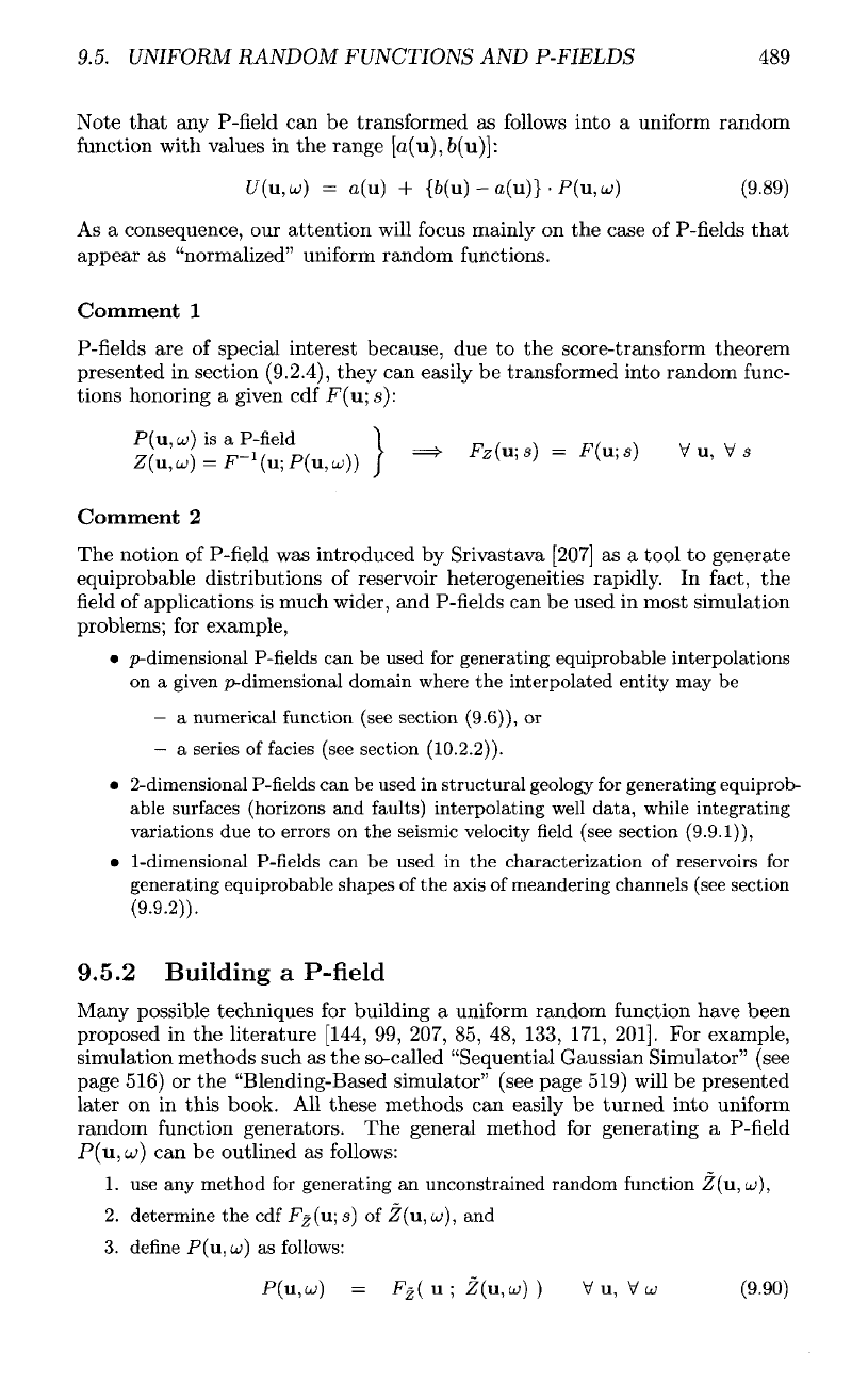
By
definition,
• The
random
function
C/(u,
u>)
is a
Uniform
Random
Function
(URF)
if its cdf
FU
(u;
s) is
such
that
where
U(s
a(u),6(u))
is the
uniform
cdf
denned
on
[a(u),6(u)]
by
equation
(9.11),
while
a(u)
and
6(u)
are two
given
functions
such
that
• The
random
function
P(u,
u;)
is a
P-field
34
if it is a
uniform
random
function
distributed
on
[0,1],
that
is to
say,
if its cdf
Fp(u;p)
is
such
that
34
The
name
"P-field,"
an
acronym
for
"Probability-field," comes
from
the
fact
that,
similarly
to
probabilities,
P-fields
have values
in the
range
[0,1].
9.5.
UNIFORM
RANDOM FUNCTIONS
AND
P-FIELDS
489
Note
that
any
P-field
can be
transformed
as
follows
into
a
uniform
random
function
with values
in the
range
[a(u),&(u)j:
As
a
consequence,
our
attention
will
focus
mainly
on the
case
of
P-fields
that
appear
as
"normalized"
uniform
random
functions.
Comment
1
P-fields
are of
special interest because,
due to the
score-transform theorem
presented
in
section
(9.2.4),
they
can
easily
be
transformed into random
func-
tions honoring
a
given
cdf
F(u;
s):
Comment
2
The
notion
of
P-field
was
introduced
by
Srivastava [207]
as a
tool
to
generate
equiprobable
distributions
of
reservoir heterogeneities rapidly.
In
fact,
the
field
of
applications
is
much
wider,
and
P-fields
can be
used
in
most simulation
problems;
for
example,
•
p-dimensional P-fields
can be
used
for
generating equiprobable interpolations
on
a
given p-dimensional domain where
the
interpolated entity
may be
—
a
numerical function (see
section
(9.6)),
or
—
a
series
of
facies
(see section (10.2.2)).
•
2-dimensional P-fields
can be
used
in
structural geology
for
generating equiprob-
able surfaces (horizons
and
faults) interpolating well
data,
while integrating
variations
due to
errors
on the
seismic velocity
field
(see section (9.9.1)),
•
1-dimensional P-fields
can be
used
in the
characterization
of
reservoirs
for
generating equiprobable shapes
of the
axis
of
meandering channels (see section
(9.9.2)).
9.5.2
Building
a
P-field
Many
possible techniques
for
building
a
uniform
random
function
have been
proposed
in the
literature [144,
99,
207,
85, 48,
133, 171, 201].
For
example,
simulation
methods such
as the
so-called "Sequential Gaussian Simulator" (see
page
516)
or the
"Blending-Based simulator" (see page 519)
will
be
presented
later
on in
this
book.
All
these
methods
can
easily
be
turned into uniform
random
function
generators.
The
general method
for
generating
a
P-field
.P(u,
w)
can be
outlined
as
follows:
1. use any
method
for
generating
an
unconstrained random function
Z(u,u>),
2.
determine
the cdf
F^(u;
s) of
Z(u,
a>),
and
3.
define
P(u,
cu)
as
follows:
490
CHAPTER
9.
STOCHASTIC MODELING
According
to the
score-transform theorem presented
in
section
(9.2.4),
the
random
function
P(u,
u;)
so
defined
has a cdf
function
corresponding
to a
uniform
distribution
on
[0,1]:
In
practice,
the
covariance
function
CjK
u
i
>
U2
)
°f
the
random
function
Z(u,
a;)
can be
selected
in
many
different
ways, depending
on the
context
of the
sim-
ulation problem (see section
(9.6)).
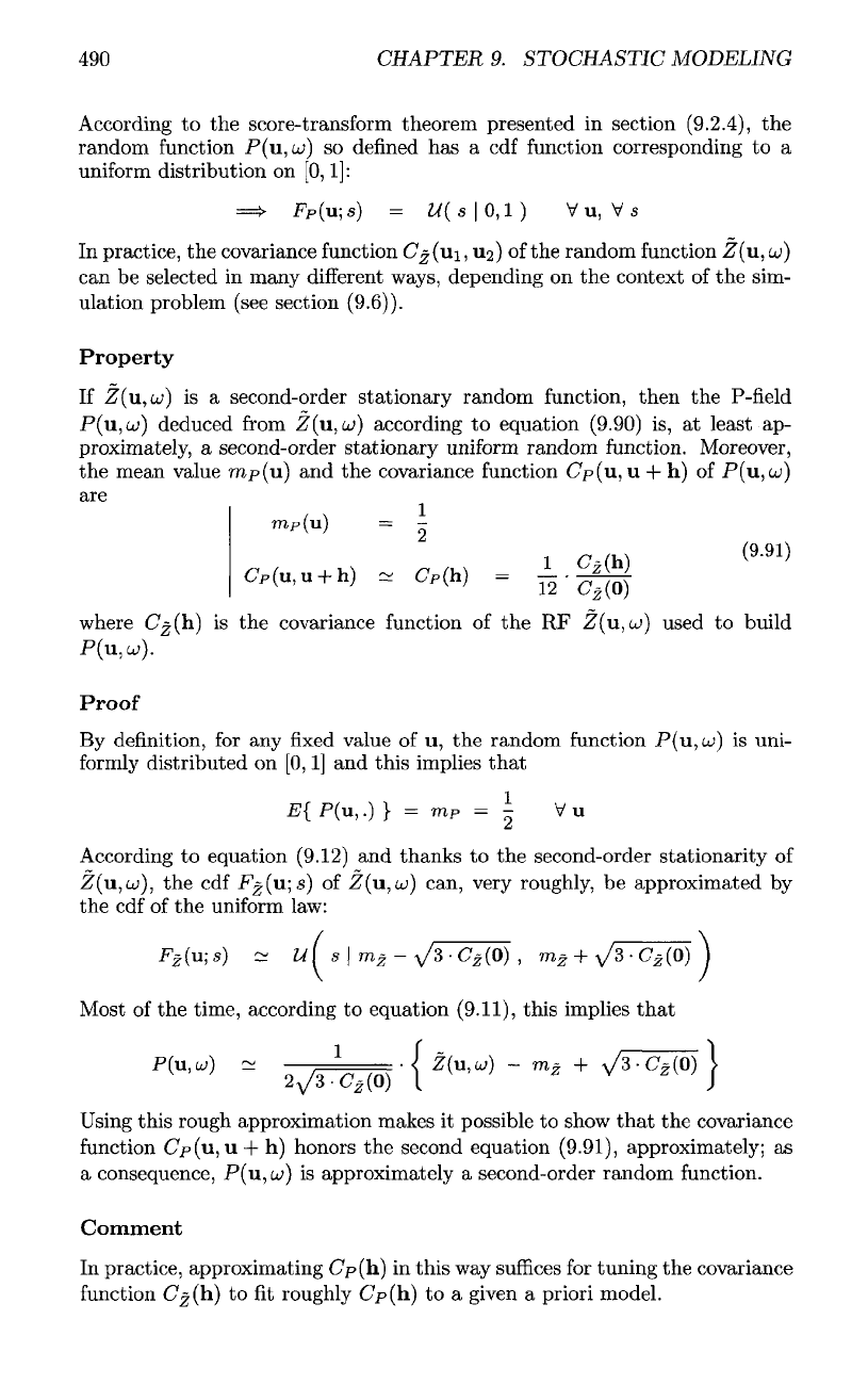
Property
If
Z(u,ijj)
is a
second-order stationary random
function,
then
the
P-field
P(u,u)
deduced
from
Z(u,u)
according
to
equation
(9.90)
is, at
least
ap-
proximately,
a
second-order
stationary
uniform
random
function. Moreover,
the
mean value
rap(u) and the
covariance
function
(7p(u,
u + h) of
P(u,
u;)
are
where
Cjj(h)
is the
covariance
function
of the RF
Z(u,cj)
used
to
build
P(u,u;).
Proof
By
definition,
for any fixed
value
of u, the
random
function
P(u,
o>)
is
uni-
formly
distributed
on
[0,1]
and
this implies
that
According
to
equation
(9.12)
and
thanks
to the
second-order stationarity
of
2T(u,
w),
the cdf
F^(u;s)
of
Z(u,a;)
can, very roughly,
be
approximated
by
the
cdf
of the
uniform
law:
Most
of the
time, according
to
equation (9.11),
this
implies
that
Using
this rough approximation makes
it
possible
to
show
that
the
covariance
function
Cp(u,
u + h)
honors
the
second equation (9.91), approximately;
as
a
consequence,
P(u,
u) is
approximately
a
second-order random function.
Comment
In
practice, approximating
Cp(la)
in
this
way
suffices
for
tuning
the
covariance
function
C^(h)
to fit
roughly
Cp(h)
to a
given
a
priori model.
9.5.
UNIFORM
RANDOM FUNCTIONS
AND
P-FIELDS
9.5.3
Theorem
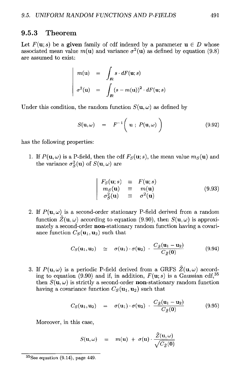
Let
-F(u;
s) be a
given
family
of cdf
indexed
by a
parameter
u
G D
whose
associated mean value m(u)
and
variance
cr
2
(u)
as
defined
by
equation (9.8)
are
assumed
to
exist:
Under
this condition,
the
random
function
S(u,
u;)
as
defined
by
has the
following
properties:
1.
If
P(u,
a;)
is a
P-field,
then
the cdf
-Fg(u;
s), the
mean value
ras(u) and
the
variance
cr|(u)
of
S(u,aj)
are
2.
If
P(u,
u))
is a
second-order stationary
P-field
derived
from
a
random
function
Z(u,cu)
according
to
equation
(9.90),
then
S(u,uj)
is
approxi-
mately
a
second-order
non-stationary
random function having
a
covari-
ance
function
Cs(ui,ii2)
such
that
3.
If
P(u,
u))
is a
periodic
P-field
derived
from
a
GRFS
Z(u,w)
accord-
ing
to
equation
(9.90)
and if, in
addition,
F(u;
s)
is a
Gaussian
cdf,
35
then
5(u,
u;)
is
strictly
a
second-order
non-stationary
random function
having
a
covariance
function
€3(111,112)
such
that
Moreover,
in
this
case,
35
See
equation (9.14), page 449.
491
492
CHAPTER
9.
STOCHASTIC
MODELING
Proof
It can be
observed
that
•
equation
(9.93)
is a
direct
consequence
of the
score-transform
theorem
(see
equation
(9.17))
and
definitions
(9.88)
and
(9.92).
•
equations
(9.94)
is a
straightforward
consequence
of the
approximation
(9.13)
and
properties
(9.91)
and
(9.89).
Let us now
assume
that
P(u,
o>)
is the
periodic
P-field
denned
in
section
(9.5.2)
and
that
F(u;
s)
is a
Gaussian cdf:
It can be
observed
that,
for any p G
[0,1],
Taking into account condition (9.73)
and
equations
(9.92)
or
(9.90),
it can be
deduced
that
where
Z(u,u;)
is the
GRFS used
to
build
P(U,UJ).
From this equation,
it can be
concluded
that
5(u,
a;)
is a
second-order
non-stationary
RF
honoring equations
(9.95).
9.6
Stochastic simulators
As
explained
in
section
(9.1),
the
main purpose
of
this chapter
is to
propose
simulation techniques capable
of
producing equiprobable solutions
to
inter-
polation problems. These solutions
are
called "simulations"
and are
defined
as
realizations
of
random functions called "stochastic simulators"
or,
more
simply,
"simulators." Many
different
techniques have been proposed
in the
literature
for
building simulators (e.g.,
see
[215,
58,
94]).
In
this section,
havin g
denned
the
notion
of
simulator, three examples
of
particularly simple
techniques
for
building simulators
are
given. Other techniques will
be
pre-
sented
later
on in
sections
(9.7.7),
(9.7.8), (9.9.1),
and
(9.8)
and in
chapter
10 .
9.6.1
The
interpolation versus simulation problem
As
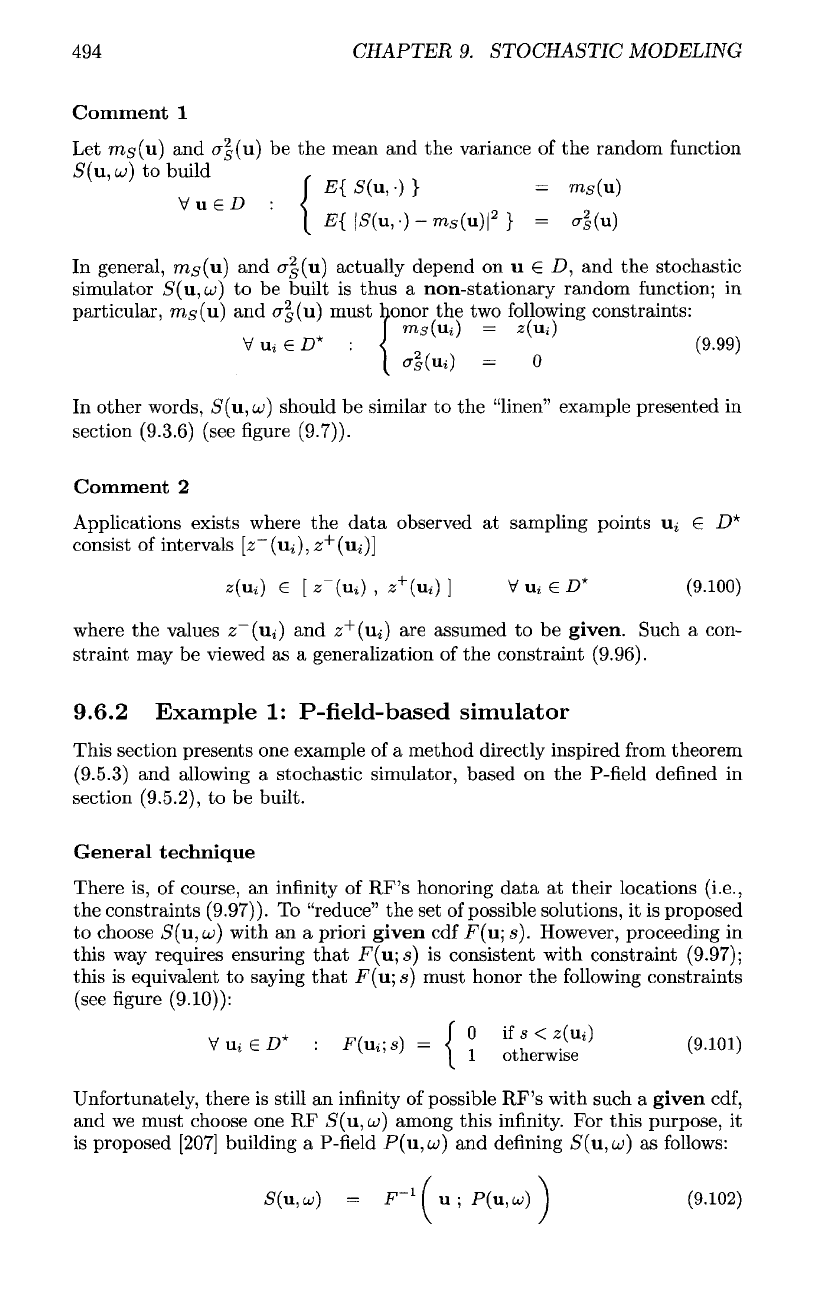
suggested
in figure
(9.10),
let
z(u)
be an
unknown
scalar
function
defined
on
a
region
D of a
normed linear vector
space
36
8
(see
[141])
and
known only
o n
a finite
subset
D*
consisting
of N
sampling
points
{ui,...,
ujv}
belonging
toD:
36
For
example,
this
space
can be the
Euclidean
parametric
space
(x,
y,
z)
or a
curvilinear
parametric
space
(u,v,w)
corresponding
to a
stratigraphic
grid
(see
figure
(10.1)).
9.6.
STOCHASTIC SIMULATORS
Figur e
9.10
The
interpolation
problem
consists
in
estimating
at
point
u
(white
dot)
a
function
z(u)
denned
on a
part
D of a
normed
linear
vector
space
E and
known
at a finite set
of
N
sampling
points
{ui}
(black
dots).
In
practice,
sampling
data
points
may be
limited
to a
neighborhood
W(u)
of
point
u.
With such limited information, there
are two
possible strategies
for
assessing
the
variations
of
z(u)
on D:
• The first
strategy
involves
looking
for a
unique
function
z*(u)
defined
on D
and
assumed
to
interpolate
the
unknown
function
2(11)
on
D*:
In
this
case,
z*(\i)
is
assumed
to be
built
to
provide
the
"best"
solution.
37
• The
second
strategy
consists
of
looking
for a
random
function
S^u,
u;)
defined
on
D and
assumed
to
have
all its
realizations equiprobable
and
constrained
to
interpolate
z(u)
on
D*:
In
practice, these
two
strategies
are
complementary,
and
section
(9.6.2)
will
show
how any
interpolator
z*(u)
can be
used
for
building such
a
random
function
S(u,u;).
If
one
succeeds
in
building such
an RF
S(u,
cu),
then,
to any
series
{uji,
u^,
•
•
•}
of
equiprobable statistical elementary events,
a
series
of
equiprobable realiza-
tions
{z*(u),
z%(u),...}
interpolating
the
initial
data
can be
associated:
By
definition,
the
functions
{Zj(u)}
so
generated
are
called
the
"simulations"
of
the
unknown
function
z(u)
and the
associated random
function
S^u,
uj]
is
called
a
(stochastic) "simulator."
37
The
notion
of
"best" solution
has to be
denned
with regard
to a
specific
goodness
criterion
depending
on the
interpolation technique.
493
494
CHAPTER
9.
STOCHASTIC MODELING
Comment
1
Let
ras(u) and
cr|(u)
be the
mean
and the
variance
of the
random
function
5(11,0;)
to
In
general,
ms(u)
and
cr|(u)
actually depend
on
u
e
D,
and the
stochastic
simulator
5(11,0;)
to be
built
is
thus
a
non-stationary
random
function;
in
particular,
ras(u) and
cr|(u)
must honor
the two following
constraints:
In
other words,
5(u,o;)
should
be
similar
to the
"linen" example presented
in
section
(9.3.6)
(see
figure
(9.7)).
Comment
2
Applications
exists where
the
data
observed
at
sampling points
u^
6
D*
consist
of
intervals
[z~(u^),
z
+
(u^)]
where
the
values
z~(ui)
and
z
+
(ui)
are
assumed
to be
given.
Such
a
con-
straint
may be
viewed
as a
generalization
of the
constraint (9.96).
9.6.2
Example
1:
P-field-based
simulator
This section presents
one
example
of a
method directly inspired
from
theorem
(9.5.3)
and
allowing
a
stochastic simulator, based
on the
P-field
defined
in
section (9.5.2),
to be
built.
General
technique
There
is, of
course,
an
infinity
of
RF's honoring data
at
their locations
(i.e.,
the
constraints
(9.97)).
To
"reduce"
the set of
possible solutions,
it is
proposed
to
choose
5(u,a;)
with
an a
priori
given
cdf
-F(u;
s).
However, proceeding
in
this
way
requires ensuring
that
F(u;
s]
is
consistent with constraint
(9.97);
this
is
equivalent
to
saying
that
F(u;
s]
must honor
the
following
constraints
(see
figure
(9.10)):
Unfortunately,
there
is
still
an
infinity
of
possible RF's with such
a
given
cdf,
and we
must choose
one RF
5(u,
uj]
among this
infinity.
For
this purpose,
it
is
proposed [207] building
a
P-field
P(u,o;)
and
defining
5(u,o;)
as
follows:
build
9.6.
STOCHASTIC SIMULATORS
According
to the
theorem
in
section
(9.5.3) page
491,
the cdf
F$(u;
s) of the
RF
S(u]
a;)
so
defined
is
identical
to
F(u;
s)
Moreover,
according
to
this theorem, choosing
a
second-order stationary
ran-
dom
function
for
P(u,
u)
implies
that
S(u;
a;)
is
approximately
a
second-order
random function having
a
covariance
function
(7s(ui,
112)
such
that
In
this expression,
cr|(u)
represents
the
variance
of
S(u,u),
while
C^(h)
is
the
stationary
covariance
function
of the RF
Z(u,
u]
used
to
build
the
P-field
P(u,u;)
(see
section
(9.5.2)).
It
should
be
noted
that
Cs(iii,
u
2
)
does
not
change
if the
covariance
func-
tion
C^(h)
is
multiplied
by a
constant.
In
other words,
in
addition
to the
data
configuration,
only
the
type
and the
range
of the
covariance
function
C^(h)
can
have
an
influence
on
Cs(ui,u
2
)
and
thus
on the
simulator
S(u,u>).
From this observation
and
according equations
(9.94)
and
(9.95),
it can
be
concluded
that
•
erf
(u)
controls
the
amplitude
of the
variations
of
£(11,0;);
•
CZ(\\}/CZ(Q]
controls
the
style
of the
variations
of
S^u,a;).
Comment
1
Sections
(9.7.7)
and
(9.9.1)
present situations where
it is
possible
to
choose
F(u;
s] in
such
a way
that
the
associated variance
cr|(u)
honors
the
following
constraint:
u far
away
from
the
data
points
In
this case, equation (9.104)
can be
simplified
to
obtain
{
Ui
far
away
from
the
data points
^
112
far
away
from
the
data points
J
As
a
consequence,
if
constraint
(9.105)
is
honored,
and if we
move
far
away
from
the set
D*
of the
data
points, then, taking into account equations (9.106)
and
(9.70),
it can be
said
that
Cj,(h)
directly controls
• the
behavior
of the
simulator
S(u,
o>),
and
• the
style
of
each
simulation
Zj(u)
=
5(u,to,-).
From this observation,
it is
deduced
that,
if
S(u,u)
is
required
to
have
a
given
stationary covariance
function
cov(h)
when
far way
from
the
data
points, then
one
must choose
Comment
2
In
the
case
of
interval
data
types corresponding
to
constraint
(9.100),
a cdf
honoring
the
following
constraints, which generalize
the
constraints (9.101),
is all that has to be chosen for F(u: s}:
495
496
CHAPTER
9.
STOCHASTIC MODELING
Comment
3
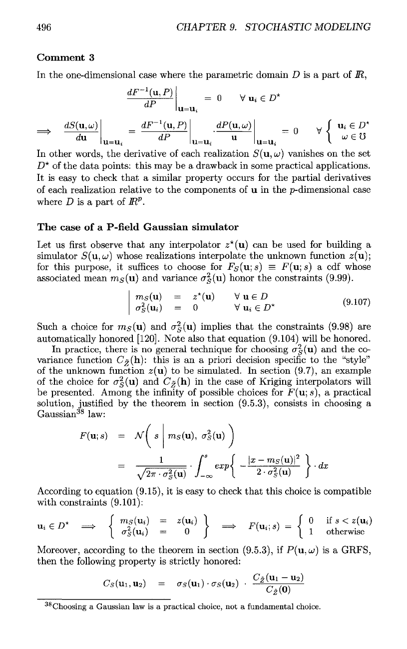
In
the
one-dimensional case where
the
parametric domain
D is a
part
of
iR,
In
other words,
the
derivative
of
each realization
5(11,
u;)
vanishes
on the set
D*
of the
data
points: this
may be a,
drawback
in
some practical applications.
It is
easy
to
check
that
a
similar property occurs
for the
partial derivatives
of
each realization relative
to the
components
of u in the
p-dimensional
case
where
D is a
part
of
1R
P
.
The
case
of a
P-field
Gaussian
simulator
Let
us first
observe
that
any
interpolator
z*(u)
can be
used
for
building
a
simulator
5(u,o;)
whose realizations interpolate
the
unknown
function
z(u);
for
this
purpose,
it
suffices
to
choose
for
FS(U;S)
=
F(u;s)
a cdf
whose
associated mean
ms(u)
and
variance
cr|(u)
honor
the
constraints
(9.99).
Such
a
choice
for
7715(u)
and
cr|(u)
implies
that
the
constraints (9.98)
are
automatically honored
[120].
Note also
that
equation (9.104) will
be
honored.
In
practice, there
is no
general technique
for
choosing
<r|(u)
and the co-
variance
function
C^(h):
this
is an a
priori decision
specific
to the
"style"
of
the
unknown
function
z(u)
to be
simulated.
In
section
(9.7),
an
example
of
the
choice
for
cr|(u)
and
Cjj(h)
in the
case
of
Kriging interpolators will
be
presented. Among
the
infinity
of
possible choices
for
jF(u;s),
a
practical
solution,
justified
by the
theorem
in
section
(9.5.3),
consists
in
choosing
a
Gaussian
38
law:
According
to
equation
(9.15),
it is
easy
to
check
that
this choice
is
compatible
with
constraints
(9.101):
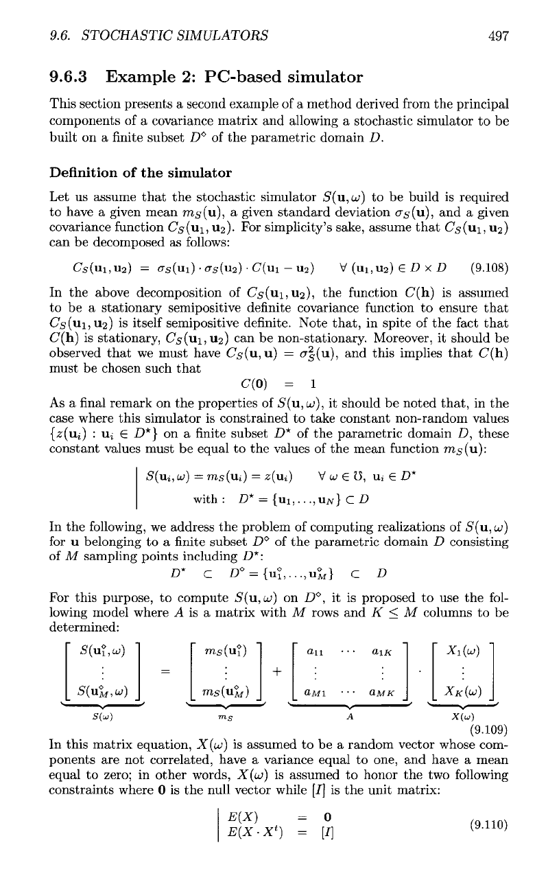
Moreover,
according
to the
theorem
in
section (9.5.3),
if
P(u,a;)
is a
GRFS,
then
the
following
property
is
strictly honored:
38
Choosing
a
Gaussian
law is a
practical choice,
not a
fundamental choice.
9.6.
STOCHASTIC SIMULATORS
9.6.3
Example
2:
PC-based simulator
This section presents
a
second example
of a
method derived
from
the
principal
components
of a
covariance matrix
and
allowing
a
stochastic simulator
to be
built
on a finite
subset
D
0
of the
parametric domain
D.
Definition
of the
simulator
Let
us
assume
that
the
stochastic simulator
5(u,
a;)
to be
build
is
required
to
have
a
given mean
ras(u), a
given
standard
deviation
as
(u),
and a
given
covariance
function
Cs(ui,
112).
For
simplicity's sake, assume
that
(7s
(ui,
u
2
)
can be
decomposed
as
follows:
In the
above decomposition
of
GS^UI,
u
2
),
the
function
C(h)
is
assumed
to be a
stationary semipositive
definite
covariance
function
to
ensure
that
(7,5(111,112)
is
itself semipositive
definite.
Note
that,
in
spite
of the
fact
that
C(h)
is
stationary,
65(111,112)
can be
non-stationary. Moreover,
it
should
be
observed
that
we
must have
Cs(u,
u)
=
cr|(u),
and
this implies
that
C(h)
must
be
chosen such
that
As
a final
remark
on the
properties
of
5(u,
u;),
it
should
be
noted
that,
in the
case
where this simulator
is
constrained
to
take constant non-random values
{z(ui)
:
Ui
€
D*}
on a finite
subset
D* of the
parametric domain
D,
these
constant
values must
be
equal
to the
values
of the
mean
function
ms
(u):
In the
following,
we
address
the
problem
of
computing realizations
of
S'(u,
a;)
for
u
belonging
to a finite
subset
D®
of the
parametric domain
D
consisting
of
M
sampling points including
D*:
For
this purpose,
to
compute
5(u,
a;)
on
jD°,
it is
proposed
to use the
fol-
lowing
model where
A is
&
matrix with
M
rows
and K
<
M
columns
to be
determined:
In
this
matrix equation,
X(u>)
is
assumed
to be a
random vector whose com-
ponents
are not
correlated, have
a
variance equal
to
one,
and
have
a
mean
equal
to
zero;
in
other words,
X(cu)
is
assumed
to
honor
the two
following
constraints where
0 is the
null vector while
[/] is the
unit matrix:
497
