Jean-Laurent Mallet. Geomodeling
Подождите немного. Документ загружается.

508
CHAPTER
9.
STOCHASTIC MODELING
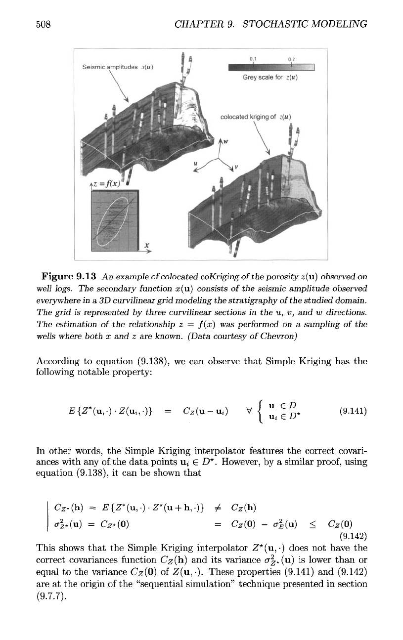
Figure
9.13
An
example
ofcolocated
coKriging
of
the
porosity
z(u)
observed
on
well
logs.
The
secondary
function
x(u)
consists
of the
seismic
amplitude
observed
everywhere
in a 3D
curvilinear
grid
modeling
the
stratigraphy
of
the
studied
domain.
The
grid
is
represented
by
three
curvilinear
sections
in the u, v, and
w
directions.
The
estimation
of the
relationship
z =
f(x)
was
performed
on a
sampling
of the
wells
where
both
x and z are
known.
(Data
courtesy
of
Chevron)
According
to
equation
(9.138),
we can
observe
that
Simple Kriging
has the
following
notable property:
In
other words,
the
Simple Kriging interpolator features
the
correct covari-
ances with
any of the
data
points
iij
G
D*.
However,
by a
similar
proof,
using
equation
(9.138),
it can be
shown
that
This shows
that
the
Simple Kriging interpolator
Z*(u,
•)
does
not
have
the
correct covariances
function
Cz(h)
and its
variance
cr|*(u)
is
lower
than
or
equal
to the
variance
Cz(0)
of
Z(u,
•).
These properties (9.141)
and
(9.142)
are at the
origin
of the
"sequential simulation" technique presented
in
section
(9.7.7).
9.7.
KRIGING-BASED
METHODS
5
9.7.4
Colocated
coKriging
As
suggested
in figure
(9.13),
let us
assume
that
the
function
z(u)
to be
interpolated
is
linked
by a
functional
relationship
to a
second
function
44
x(u)
assumed
to be
known everywhere
on
D:
Unfortunately,
due to
measurement errors, this link
is not
fully
reliable
and
should
be
considered only
as a
hint
as to the
behavior
of
z(u)
when
a
long
way
from
the
data
points. Several geostatistical methods, called coKriging [224,
80]
or
Colocated Kriging
[237],
have been proposed
for
taking into account
this
"fuzzy"
link between
z(u)
and
x(u).
A
complete presentation
of
these
methods
is
beyond
the
scope
of
this book,
but a
very simple alternative
to
colocated coKriging
can be
formulated
as
follows:
where
•
z*(u)
is
either
an
ordinary
or
Simple Kriging
interpolator;
• p is a
given
"certainty
factor"
belonging
to
[0,1],
which
is
used
to
weight
the
importance
of the
functional link (9.143)
relative
to the
result
z*(u)
yielded
by
the
Kriging
interpolator
£*(u);
and
•
cr|;(u)
is the
estimation
variance
associated
with
z*(u).
Let
us
assume
that
the
covariance
function
C^(h)
used
for
building
the Or-
dinary Kriging interpolator
z*(u)
is
such
45
that
Taking into account
the
properties shown
in
equations
(9.134),
(9.135),
(9.137),
and
(9.140),
it is
easy
to
check
that
z*(u)
so
defined
is
also
an
exact interpo-
lator behaving
as
follows:
• in the
neighborhood
of a
data
point
u^,
the
value
z*
p
(u)
is
close
to the
value
z*
(u) of the
ordinary Kriging;
•
when "far" from
the
data
points,
the
estimated
value
Zp(u)
is
close
to the
value
(I-
p)-
z*(u)
+ p •
f{x(u)}.
Moreover,
according
to
equation
(9.144),
it is
clear
that
the
certainty factor
p
controls
the
importance
of
f{x(u)}
relative
to
z*(u).
44
For
example,
in the
case
where
z(u)
represents
a
permeability,
it was
mentioned
on
page
440
that parameters
linked
to the
invariants
of the
strain tensor
(e.g.,
the
dilatation)
can be
used
as a
second
function
x(u)
correlated
to
2(11).
An
other example
of
functions
that
can
be
correlated
to
z(u)
are
"seismic attributes," consisting
of
local weighted combinations
of
seismic
amplitudes.
45
This
is the
case
for all the
covariance
function
models presented
on
page 464.
50
510
CHAPTER
9.
STOCHASTIC MODELING
Comment
Our
presentation
of the
colocated estimator (9.144) appears more like
a
recipe
than
a
mathematical method. However,
if it is
assumed
that
there
is a
corre-
lation between
Z and
f(X)
such
that
then
it is
possible
to
show
(see
[237,
63,
45])
that
the
best linear estimation
z*(u)
of
z(u)
is
actually such
that
It
should
be
noted that,
for
small values
of
p
2
,
this estimator
is
equivalent
to
equation (9.144).
9.7.5
Practical implementation techniques
Window
W(u)
It can be
seen
that
the
size
of the
linear systems (9.132)
and
(9.138) corre-
sponding
to the
Kriging equations
is
proportional
to the
number
TV
of
sampling
points. This implies
that
the CPU
time
for
solving this system
on a
computer
is
proportional
to
TV
2
(see
[177]).
On the
other hand,
in
practice,
it can be
observed
that
• in the
case
of
Simple Kriging,
the
weighting
coefficients
(Ai(u)}
become
negli-
gible
as
soon
as the
distance
||uj
—
u||
is
larger
that
the
range
of the
covariance
function
(or the
variogram)
in the
(uj
—
u)
direction;
and
• if
A
7
"
is
large,
e.g.,
greater
than
100,
numerical
errors
may
become
a
major
concern when resolving
the
linear
system
(9.132).
Therefore,
as
suggested
in figure
(9.10),
a
better strategy widely used
in
geo-
statistics consists
of
limiting
the
data
used
in
equation (9.132)
to the
subset
of
sampling points located
in a
window
W(u)
centered
on the
point
u
where
z(u)
has to be
estimated.
In
practice, this window consists
of an
ellipsoid
centered
on u
whose radius
p(d)
in the d
direction
is
greater
than
or
equal
to
the
radius
of the
ellipsoid
defining
the
range
of the
covariance
function
or the
variogram
in
this direction (see page 464).
In the
case where
W(u)
is cut by
a
discontinuity
(e.g.,
a
fault
[154]),
it is
recommended
to
truncate
it in
such
a way
that
its
interior remains
on the
same side
of the
discontinuity
as u.
This "divide
and
conquer" strategy
is
very
efficient
as
long
as the
following
condition
is
honored
where
D*(u)
represents
the
points
of D*
located
in
W(u).
However,
it is
relevant
to
note
that
strongly clustered
data
points,
as is
often
the
case
in
geoscience,
46
may
lead
to
this condition
not
being honored.
In
this case
the
46
For
example, this
is the
case
for
data
collected
on
well
logs.
9.7.
KRIGING-BASED
METHODS
5
local Kriging approach
may
generate irrelevant discontinuities
for
z*(u)
and
some
specific
precautions have
to be
taken
(e.g.,
see
[94],
p.
178).
Normal
score-transform
Using
a
normal score-transform (see page 470)
in
association with
the
Kriging
methods
is a
common practice discussed
in
this section.
According
to
equation
(9.53),
the cdf
-F^(u;
z)
associated with
the
normal
score-transform
Z(u,
a;)
of the
random
function
Z(u,
u)
is a
Gaussian cdf.
On
the
other hand,
the
truth
of the
following
implication
can
easily
be
checked:
Gaussian
Gaussian
FZ(U,UI,..
.,ujv;z,zi,..
.,ZN)
Gaussian
Gaussian
Assuming
-F^(u,
ui,...,
UTV;
z,
zi,...,
ZTV)
to be
Gaussian
47
is
thus compatible
with
the
normal score-transform
and
makes
it
possible
to
benefit
from
the
properties
of the
multivariate Gaussian
law
(see page 453):
• as a
linear
combination
of the
Random
Variables
{Z(ui,u)},
the
Kriging
estimator
Z*(u,
u>)
is a
Gaussian
variable;
and
•
among
all the
possible
linear
or
nonlinear
estimations
of
Z(u,
o>),
the
linear
estimator
Z*(u,
u;)
yielded
by the
Kriging
equations
is the one
that
realizes
the
lowest
minimum
for the
estimation
variance.
In
other words, proceeding
as
suggested
by
this schema
enables
an
optimal estimator
z*(u),
which
is now a
nonlinear
function
of the
initial
data
(z(ui),...,
Z(UAT)},
to be
obtained.
However,
in
general,
the
variance
of
estimation
cr|,(u)
of
Z(u,
a;)
is
different
from
the
inverse transform
of the
variance
of
estimation
crf;(u)
of
Z(u,
u?):
Much
worse, generally
the
estimator
Z*(u,
u;)
so
obtained
is
biased
[115]:
47
This
is not a
hypothesis,
but a
model
very
similar
to
choosing
the
degree
of a
polyno-
mial
if
using
a
spline
or
Bezier
interpolation.
51
512
CHAPTER
9.
STOCHASTIC MODELING
9.7.6
About
the
Heisenberg uncertainty principle
Within
the
framework
of
particle physics,
the
Heisenberg uncertainty principle
tells
us
that
From
the
same
set
of
data,
either
position
or
momentum
of
a
particle
can
be
measured
with
precision.
It can be
observe
that,
in the
frame
of our
interpolation problem,
z(u)
is the
analog
of the
position
of a
particle while
the
standard deviation
of the
estimate
of
z(u)
is the
analog
of its
momentum. Since Kriging yields both
an
estimate
z*
(u) and a
variance
of
estimation
a\,
(u),
one may be
tempted
to
claim
that
traditional Kriging methods
do not
suffer
from
a
similar uncertainty principle.
In
fact,
such
a
naive interpretation
of
Kriging makes
the
implicit assumption
that
a\
(u)
measures
the
precision
on the
estimate
z*
(u).
Unfortunately,
this
implicit assumption
is not
true because
it can
only
be
said
that
<r|;(u)
is no
more
than
a
"pseudo-distance"
to
data
locations, which
is
independent
of the
actual values
of
these
data.
It
should
be
noted, however,
that
if a
second
set of
data
independent
of
the first one
used
for
computing
a
Kriging estimation
is
available, then
the
exact Kriging error
can be
computed
at
these
new
data
locations: these
true errors
can
then
be
used
for
approximating
the
true variance
cr
2
(u)
as a
function
of the
variance
of
estimation
o~^
(u).
Unfortunately,
in
practice such
a
second
data
set is
generally
not
available
and
this
is why
simulation methods
must
be
used when
one
want
to
assess uncertainties.
9.7.7
P-field-based
and
PC-based simulators revisited
As an
epilogue
of
section
(9.6),
this section shows
how
P-field
and
PC-based
simulators
can be
derived
from
a
Kriging interpolation
z*(u)
of the
unknown
function
z(u)
to be
simulated
on a
parametric domain
D. In
accordance with
previous notations,
in
this section
D*
represents
a finite set of
interpolation
points belonging
to D
where
the
values
of the
function
z(u)
are
assumed
to
be
given.
Preliminary
remark
Note
that,
according
to
equations (9.107),
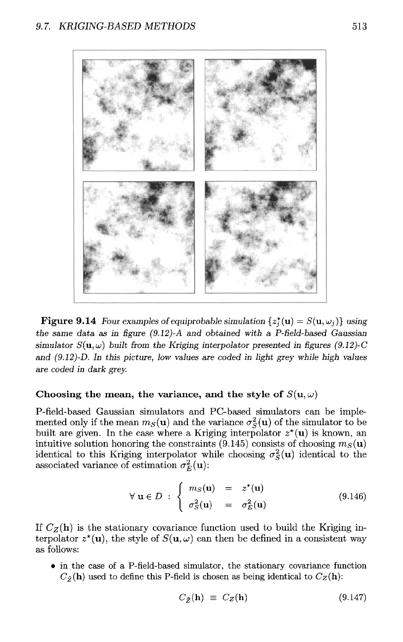
any
simulator
5(11,0;)
is a
nonsta-
tionary random
function
honoring
the
following
constraint:
This
clearly shows
that
S(u,
u;)
cannot
be
identical
to the
stationary random
function
Z(u,
o;)
used to
define
the Kriging interpolator (see equation
(9.125))
whose
stationary mean
and
variance
are
such
that
9.7.
KRIGING-BASED
METHODS
513
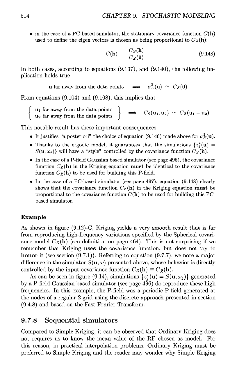
Figure
9.14
Four
examples
of
equiprobable
simulation
{z*(u)
=
5(11,
cjj)}
using
the
same
data
as in figure
(9.12)-A
and
obtained
with
a
P-field-based
Gaussian
simulator
£(11,01)
built
from
the
Kriging
interpolator
presented
in figures
(9.12)-C
and
(9.12)-D.
In
this
picture,
low
values
are
coded
in
light
grey
while
high
values
are
coded
in
dark
grey.
Choosing
the
mean,
the
variance,
and the
style
of
S(u,uj]
P-field-based
Gaussian simulators
and
PC-based simulators
can be
imple-
mented only
if the
mean
ms
(u) and the
variance
cr|
(u)
of the
simulator
to be
built
are
given.
In the
case where
a
Kriging interpolator
z*(u)
is
known,
an
intuitive
solution honoring
the
constraints
(9.145)
consists
of
choosing
ra,s(u)
identical
to
this Kriging interpolator while choosing
cr|(u)
identical
to the
associated variance
of
estimation
cr|n(u):
If
Cz(h)
is the
stationary covariance
function
used
to
build
the
Kriging
in-
terpolator
z*(u),
the
style
of
5(u,
a;)
can
then
be
defined
in a
consistent
way
as
follows:
• in the
case
of a
P-field-based
simulator,
the
stationary
covariance
function
C^(h)
used
to
define
this
P-field
is
chosen
as
being
identical
to
Cz(h):
514
CHAPTER
9.
STOCHASTIC MODELING
• in the
case
of a
PC-based
simulator,
the
stationary
covariance
function
C(h)
used
to
define
the
eigen
vectors
is
chosen
as
being
proportional
to
Cz(h):
In
both cases, according
to
equations
(9.137),
and
(9.140),
the
following
im-
plication holds true
u far
away
from
the
data
points
From equations (9.104)
and
(9.108),
this
implies
that
{
Ui
far
away
from
the
data points
1
U2
far
away
from
the
data
points
J
This
notable result
has
these important consequences:
• It
justifies
"a
posteriori"
the
choice
of
equation
(9.146)
made
above
for
erf
(u).
•
Thanks
to the
ergodic
model,
it
guarantees
that
the
simulations
{^(u)
=
S(u,u>j)}
will
have
a
"style"
controlled
by the
covariance
function
Cz(h).
• In the
case
of a
P-field
Gaussian
based
simulator
(see
page
496),
the
covariance
function
Cz(h)
in the
Kriging
equation
must
be
identical
to the
covariance
function
C^(ti)
to be
used
for
building
this
P-field.
• In the
case
of a
PC-based
simulator
(see
page
497),
equation
(9.148)
clearly
shows
that
the
covariance
function
Cz(h)
in the
Kriging
equation
must
be
proportional
to the
covariance
function
C(h)
to be
used
for
building
this
PC-
based
simulator.
Example
As
shown
in
figure
(9.12)-C,
Kriging yields
a
very smooth result
that
is far
from
reproducing high-frequency variations specified
by the
Spherical covari-
ance model
Cz(h)
(see definition
on
page 464).
This
is not
surprising
if we
remember
that
Kriging
uses
the
covariance
function,
but
does
not try to
honor
it
(see section
(9.7.1)).
Referring
to
equation
(9.7.7),
we
note
a
major
difference
in the
simulator
5(u,
u;)
presented above, whose behavior
is
directly
controlled
by the
input covariance
function
C^(h)
=
C^(h).
As
can be
seen
in
figure
(9.14), simulations
{Zj(u)
=
5(u,cc>j)}
generated
by
a
P-field Gaussian based simulator (see page 496)
do
reproduce these high
frequencies.
In
this example,
the
P-field
was a
periodic P-field generated
at
the
nodes
of a
regular 2-grid using
the
discrete approach presented
in
section
(9.4.8)
and
based
on the
Fast
Fourier Transform.
9.7.8
Sequential simulators
Compared
to
Simple Kriging,
it can be
observed
that
Ordinary Kriging does
not
requires
us to
know
the
mean value
of the RF
chosen
as
model.
For
this reason,
in
practical interpolation problems, Ordinary Kriging must
be
preferred
to
Simple Kriging
and the
reader
may
wonder
why
Simple Kriging
9.7.
KRIGING-BASED
METHODS
515
has
been introduced.
The
only reason
for
introducing Simple Kriging
in
this
book
is
that
it is
often
used
for
building
a
sequential simulation technique
to be
presented below.
As
will
be
seen, this sequential technique initially proposed
by
Journel
is
quite
different
from
the
P-field
approach demonstrated
up to
now.
Building
a
sequential
simulator
For
simplicity's sake,
let us
assume
that
the
simulator
S^u,
to>)
that
we
want
to
build
is
centered
and is
order
2
stationary:
Suppose
that
the
simulator
S(u,
a;)
is
already known
on a finite set
£>*
of n
sampling points:
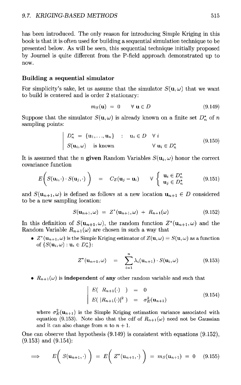
It is
assumed
that
the n
given
Random Variables
S(\ii,u))
honor
the
correct
covariance function
and
S(u
n
+i,uj)
is
defined
as
follows
at a new
location
u
n+
i
€ D
considered
to be a new
sampling location:
In
this
definition
of
S(u
n+
i,uj),
the
random
function
Z*(u
n+
i,uj}
and the
Random Variable
R
n+
i(u)
are
chosen
in
such
a way
that
•
Z*(u
n+
i,u;)
is the
Simple Kriging
estimator
of
Z(u,ui)
=
S(u,uj)
as a
function
of{S(ui,u)
:u
i
£Dt
l
}:
•
Rn+i(uj)
is
independent
of any
other
random
variable
and
such
that
where
crf;(u
n
+i)
is the
Simple
Kriging
estimation
variance
associated
with
equation
(9.153).
Note
also
that
the cdf of
R
n+
i(uj)
need
not be
Gaussian
and
it can
also
change
from
n to n +
1.
One
can
observe
that
hypothesis
(9.149)
is
consistent with equations
(9.152),
(9.153)
and
(9.154):
516
CHAPTER
9.
STOCHASTIC MODELING
Moreover,
taking into account
the
independence
of the
Random Variables
Rn+i(u})
and
from
equations
(9.152)
and
(9.141),
it can
easily
be
deduced
that
In
other words,
S(u
n
_|_i,a;)
as
denned
by
equation
(9.152)
honors
the
correct
covariances with
any of the
Random Variables
(5(u^,o;)
:
ii;
e
D*}.
The
equation
(9.156)
justifies
using
the
following
sequential algorithm
which
is
compatible with preconditions (9.150)
and
(9.151):
//—
Sequential
simulator
algorithm
let
u
be a
given
elementary
statistical
event
let
Dn
0
be a
given
initial
set
consisting
of
no
sampling
points
where
5(u,
a>)
is
known,
let
DM
be a
given
superset
of
D*
0
consisting
of
N
sampling
points
where
S(u,
u>)
has to be
computed,
let
n = no
while(
n < N } {
•
generate
R
n
+i(u>)
•
compute
Simple
Kriging
Z*(u
n+
i,u)
=
^™
=1
A^Un+l)
•
S(Ui,u)
•
compute
S(u
n+
i,u]1
=
Z*(u
n
+i,w)
+
Rn+i(u)
•
increment
n
D*
<—
D*
n
U
{u
n+1
}
n
<—
n + \
}
II
end:
while
Sequential Gaussian simulator
(SGS)
Most
of the
time,
a
Gaussian variable
is
chosen
for
R
n+
i(ui),
and the
sequen-
tial simulation technique described above
is
called
a
"Sequential Gaussian
Simulation"
(SGS).
In
practice,
two
types
of SGS are
used:
•
Constrained
SGS
corresponds
to the
case
where
the
simulator
S(u,u)
is
assumed
to be
degenerated
on
D*
0
:
The
values
{z(ui)
:
Ui
£
-Dn
0
}
correspond
to the
sampling
data
of the
function
z(u)
to be
simulated.
The
above
constraint
guarantees
that
such
sampling
data
will
be
honored
by
each
simulation
and
that
the
simulator
S(u,
u)
gen-
erated
by the
above
sequential
algorithm
is
similar
to the
"linen"
example
presented
in
section
(9.3.6)
and figure
(9.7).
•
Unconstrained
SGS
corresponds
to the
case
where
no
data
have
been
ob-
served.
In
this
case,
the
sequential
algorithm
can be
initialized
as
follows:
9.7.
KRIGING-BASED
METHODS
5
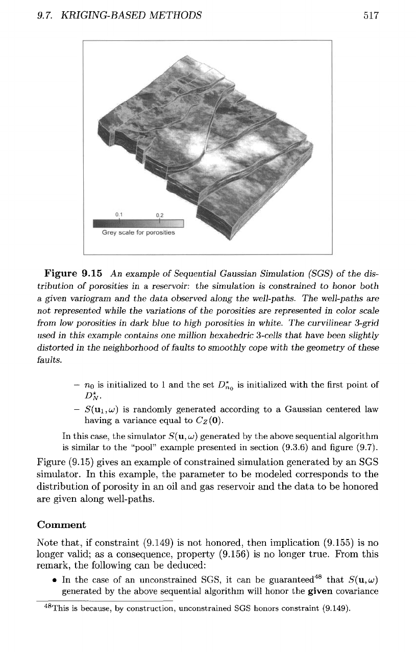
Figure
9.15
An
example
of
Sequential Gaussian Simulation (SGS)
of the
dis-
tribution
of
porosities
in a
reservoir:
the
simulation
is
constrained
to
honor
both
a
given variogram
and the
data observed along
the
well-paths.
The
well-paths
are
not
represented while
the
variations
of the
porosities
are
represented
in
color scale
from
low
porosities
in
dark blue
to
high porosities
in
white.
The
curvilinear
3-grid
used
in
this
example contains
one
million hexahedric
3-cells
that
have been slightly
distorted
in the
neighborhood
of
faults
to
smoothly cope
with
the
geometry
of
these
faults.
—
no is
initialized
to 1 and the set
D*
0
is
initialized with
the first
point
of
n*
L)
N
.
—
S(ui,u>)
is
randomly generated according
to a
Gaussian centered
law
having
a
variance equal
to
Cz(O).
In
this case,
the
simulator
<S(u,
a;)
generated
by the
above sequential algorithm
is
similar
to the
"pool" example presented
in
section (9.3.6)
and figure
(9.7).
Figure
(9.15)
gives
an
example
of
constrained
simulation
generated
by an SGS
simulator.
In
this
example,
the
parameter
to be
modeled
corresponds
to the
distribution
of
porosity
in an oil and gas
reservoir
and the
data
to be
honored
are
given
along
well-paths.
Comment
Note
that,
if
constraint
(9.149)
is not
honored,
then
implication
(9.155)
is no
longer
valid;
as a
consequence,
property
(9.156)
is no
longer
true.
From
this
remark,
the
following
can be
deduced:
• In the
case
of an
unconstrained SGS,
it can be
guaranteed
48
that
S(u,u>)
generated
by the
above sequential algorithm
will
honor
the
given
covariance
48
This
is
because,
by
construction,
unconstrained
SGS
honors
constraint
(9.149).
51
