Jean-Laurent Mallet. Geomodeling
Подождите немного. Документ загружается.

518
CHAPTER
9.
STOCHASTIC
MODELING
function
Cz(h);
• In the
case
of a
constrained SGS,
S(u,u)
is no
longer stationary.
For
this
reason,
honoring
the
given
covariance
function
C'z(h)
no
longer makes sense.
However,
in
practice,
in the
same
way as in
P-field
simulations, moving away
from
the
data
points,
it can be
observed
that
SGS
approximately reproduces
Cz(h).
P-field-based
simulators
versus
sequential
simulators
Prom
a
practical
point
of
view,
P-field-based
and
sequential
simulators
yield
similar
results
and in
several
ways
are
complementary:
• A
sequential
simulator
can be
used
to
generate
a
P-field
by
proceeding
as
follows:
—
build
an
unconstrained sequential simulator
S(u,
•)
honoring
the
speci-
fied
covariance
function
Cz(h);
and
- use the
score-transform formula (9.16)
to
build
the
P-field
P(u,
•)
where
FS(S)
is the cdf of
5(11,
•) as
follows:
•
From
the
point
of
view
of the
algorithm's
complexity,
P-field-based
and
sequential
simulators
behave
in
opposite
ways:
—
The
window
VK(u)
used
by the SGS has to be
larger than
the
range
of
the
specified
covariance
function
Cz(h).
As a
consequence,
the
bulk
of
computation needed
to
build
the
intersection
W(u)
D
D^
tends
to
increase when
the
range increases.
—
The
degree
of the
trigonometric polynomials used
for
generating periodic
P-fields
generally increases
as the
range
of
Cz(h)
decreases.
•
From
a
computer
science
point
of
view,
the
generation
of a
periodic
P-field
such
as the one
presented
in
section
(9.5.2)
can be
parallelized
in
a
straightforward way.
Conversely,
due to its
sequential
nature,
SGS
cannot
be
parallelized.
•
From
a
mathematical
point
of
view,
thanks
to
theorem
(9.5.3)
and
prop-
erty
(9.156),
both
periodic
P-fields
and
sequential-based
simulators
have
solid
fundations.
In
practice,
with
a
fairly
large
C^(h)
range,
49
periodic
P-fields
presented
in
section
(9.5.2)
are
extremely
efficient
and
must
be
preferred
to SGS for the
following
reasons:
•
they
are
faster
than
SGS;
and
49
For
example,
in a
one-dimensional problem,
the
range
R
must
be
greater
than
.D/20.
9.8.
BLENDING-BASED
METHOD
519
•
they
can be
parallelized, which dramatically increases
the
speed
of
their
computation;
In
particular, periodic
P-fields
are an
excellent choice
for
building
the
geo-
metric simulators presented
in
section (9.9.1).
Comment
It may be
that
the
function
z(u)
to be
estimated
is
correlated with another
function
x(u)
known everywhere;
for
example, this
is the
case
if
z(u)
is the
seismic
impedance observed
on
well logs, while
x(u)
represents
the
seismic
amplitude observed
in the
whole
3D
domain
of
interest.
In
such
a
situation,
a
sequential simulator could
be
built based
on
Colocated CoKriging.
It
should
also
be
mentioned
that
many other possible methods have been proposed
in
the
literature (e.g., [92,
100]).
9.8
Blending-based
method
In
this section,
a
very fast method
for
building random functions with given
mean
and
covariance functions, while honoring linear constraints
if
any,
is
proposed
[151].
This method uses
a
limited
set of
precomputed equiprobable
realizations
assumed
to be
generated
by
other
traditional
methods
and can
be
viewed
as a
"booster"
of
these traditional methods.
A
preliminary
remark
First, observe
that
the
Random Fourier Series introduced
in
section (9.4)
can
be
written
in the
following
form:
where
the
functions
(/j(u)}
are
given sine
and
cosine functions, while
the
{/%(u;)}'s
are
Random Variables adjusted
to
obtain
a
given covariance function
for
Z(u,
u;):
In
practice,
due to the
inadequacy
of
sine
and
cosine
functions,
honoring
a
given
covariance
function
cov(-,
•)
generally requires large values
for
n.
In
this section,
it
will
be
shown
that,
if
realizations
of a
given random
function
Z(u,uj)
honoring
the
covariance function
cov(-,
•) are
chosen
for
{/j(u)|
then
the
random
coefficients
{/3i(u}}
can be
chosen
in
such
a way
that,
when
n
tends toward
infinity,
Z(u,
a;)
also honors
the
same covariance
function
and
the
same linear constraints,
if
any,
as
Z(u,
w):
520
CHAPTER
9.
STOCHASTIC MODELING
The
interest
of
this approach lies
in the
fact
that,
due to the
adequacy
of
the
functions
{/j(u)j
so
chosen,
the
convergence
of
equation (9.157) toward
a
random
function
honoring constraint (9.158) occurs very rapidly
for
small
values
of
n.
According
to
equations (9.157)
and
(9.159),
Z(u,u>)
can be
seen
as a
random "blending"
of
realizations
of the
random
function
Z(u,
u}\
for
this reason,
we
propose calling
"Blending-Based
Random
Function,"
(BBRF),
the
random
function
Z(u,u;)
so
defined.
9.8.1
Notion
of
Blending-Based Random Function
Let
Z(u,
u;)
be a
random
function
for
which
the
elementary event
uj
be-
longs
to a set 0,
itself associated with
a
Probabilized Space
(0,.A,
IP}.
Let
{Z(u,
u;i(a;*)),...,
Z(u,
u
n
(u>*))}
be a
series
of n > 1
independent realizations
(see
definition
(9.28))
of
Z(u,
u;)
obtained
in the
frame
of an
n-sampling
a;*.
For
the
sake
of
simplicity
in the
following
sections,
the
events
w*
associated
with
the
sampling will
be
omitted,
and the
following
notations
will
be
used:
Let
{Bi(uj},...,
B
n
(ui)}
be a
series
of n
"blending" Random Variables associ-
ated with
the
elementary event
uj
belonging
to
15
and
honoring
the
following
constraints:
By
definition,
the
random
function
Z(u,u;)
denned
as
follows
for all u 6 D is
called
a
"Blending-Based Random Function" (BBRF):
Observe
that
Z(u,
u;)
can
also
be
written
as
follows:
9.8.
BLENDING-BASED
METHOD
5
9.8.2
Th e
BBRF
Z(u,u;),
as
defined
by
equations (9.161)
and
(9.162),
has the
following
properties:
• The
mean
and
covariance
functions
of
Z(u,
w)
are
such
that
•
When
n
tends
toward
infinity,
Z(u,
uj)
has the
same mean
and
covariance
functions
as
Z(u,u):
• If the
blending Random Variables
{Bi}
are
independent
and
have
the
same type
of
cdf, then, when
n
tends toward
infinity,
the cdf
FZ(U;S)
of
Z(U,LJ)
tends toward
a
Gaussian
cdf
having
a
mean equal
to
m^(u)
and
a
variance equal
to
C^(u,
u):
• The
blending Random Variables
{A},
as
defined
by
equation
(9.162),
have
the
following
properties where
a\.
represents
the
variance
of
$:
• If
each realization
of
Z(u,u>i)
honors
a
given linear equality constraint,
then
all the
realizations
of
Z(u,
a;)
honor
the
same equality constraint;
in
other words,
for any
domain
D,
any
real value
0, and any
distribution
X
(see
[194]),
the
following
implication holds true:
Proof
It is
relevant
to
note
that
properties (9.163)
are
straightforward consequences
of
constraints
(9.160),
which
are
assumed
to be
honored
by the
blending Ran-
dom
Variables
{B^}.
5
522
CHAPTER
9.
STOCHASTIC MODELING
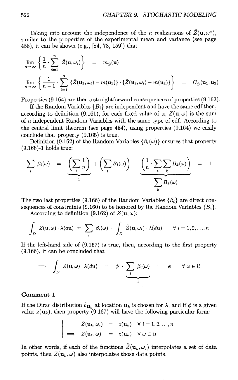
Taking into account
the
independence
of the n
realizations
of
Z(u,o;*),
similar
to the
properties
of the
experimental mean
and
variance (see page
458),
it can be
shown (e.g., [84,
78,
159])
that
Properties
(9.164)
are
then
a
straightforward consequences
of
properties
(9.163).
If
the
Random Variables
{Bi}
are
independent
and
have
the
same
cdf
then,
according
to
definition
(9.161),
for
each
fixed
value
of u,
Z(u,o;)
is the sum
of
n
independent Random Variables with
the
same type
of
cdf. According
to
the
central limit theorem (see page 454), using properties (9.164)
we
easily
conclude
that
property (9.165)
is
true.
Definition
(9.162)
of the
Random Variables
{/^(u;)}
ensures
that
property
(9.166)-1
holds true:
The two
last
properties (9.166)
of the
Random Variables
{&}
are
direct con-
sequences
of
constraints
(9.160)
to be
honored
by the
Random Variables
{Bi}.
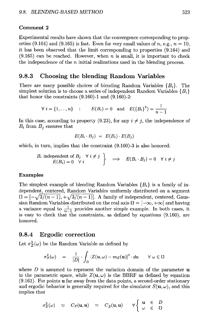
According
to
definition (9.162)
of
Z(u,
o>):
If
the
left-hand
side
of
(9.167)
is
true,
then,
according
to the first
property
(9.166),
it can be
concluded
that
Comment
1
If
the
Dirac distribution
<$u
fe
at
location
u^
is
chosen
for A, and if
^
is a
given
value
z(iifc),
then property (9.167) will have
the
following
particular
form:
In
other words,
if
each
of the
functions
Z(uk,u)i)
interpolates
a set of
data
points, then
Z(\ik,uj)
also interpolates those
data
points.
9.8.
BLENDING-BASED
METHOD
523
Comment
2
Experimental results have shown
that
the
convergence corresponding
to
prop-
erties (9.164)
and
(9.165)
is
fast. Even
for
very small values
of
n,
e.g.,
n = 10,
it
has
been observed
that
the
limit corresponding
to
properties (9.164)
and
(9.165)
can be
reached. However, when
n is
small,
it is
important
to
check
the
independence
of the n
initial realizations used
in the
blending process.
9.8.3
Choosing
the
blending Random Variables
There
are
many possible choices
of
blending Random Variables
{Bi}.
The
simplest
solution
is to
choose
a
series
of
independent
Random Variables
{Bi}
that
honor
the
constraints (9.160)-1
and
(9.160)-2:
In
this case, according
to
property
(9.23),
for any i
^
j, the
independence
of
Bi
from
Bj
ensures
that
which,
in
turn, implies
that
the
constraint
(9.160)-3
is
also honored:
Bi
independent
of Bj V i
^
j 1
E(Bi)
= 0 V i J
Examples
The
simplest example
of
blending Random Variables
{Bi}
is a
family
of in-
dependent, centered, Random Variables
uniformly
distributed
on a
segment
13
=
[—
-^/3/(n
—
1),
+y
/
3/(n
—
1)].
A
family
of
independent, centered, Gaus-
sian
Random Variables distributed
on the
real axis
O
=
[—00,
+00]
and
having
a
variance equal
to
^-j-
provides another simple example.
In
both
cases,
it
is
easy
to
check
that
the
constraints,
as
defined
by
equations
(9.160),
are
honored.
9.8.4
Ergodic correction
Let
o\((jj)
be the
Random Variable
as
defined
by
where
D is
assumed
to
represent
the
variation domain
of the
parameter
u
in
the
parametric
space,
while
Z(u,uj)
is the
BBRF
as
defined
by
equation
(9.161).
For
points
u far
away
from
the
data
points,
a
second-order stationary
and
ergodic behavior
is
generally required
for the
simulator
S(u,u}),
and
this
implies
that
524
CHAPTER
9.
STOCHASTIC MODELING
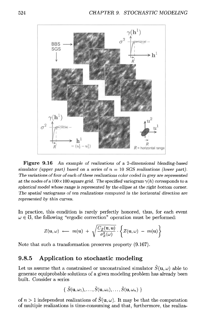
Figure
9.16
An
example
of
realizations
of a
2-dimensional
blending-based
simulator
(upper
part) based
on a
series
of
n = 10 SGS
realizations
(lower
part).
The
variations
of
four
of
each
of
these realizations color coded
in
grey
are
represented
at the
nodes
of
a
100
x 100
square grid.
The
specified
variogram
j(h)
corresponds
to a
spherical
model whose range
is
represented
by the
ellipse
at the
right
bottom
corner.
The
spatial
variograms
of
ten
realizations computed
in the
horizontal direction
are
represented
by
thin
curves.
In
practice, this condition
is
rarely perfectly honored, thus,
for
each event
<jj
€
0,
the
following
"ergodic
correction" operation must
be
performed:
Note
that
such
a
transformation preserves property
(9.167).
9.8.5
Application
to
stochastic
modeling
Let
us
assume
that
a
constrained
or
unconstrained simulator
5(u,
o>)
able
to
generate equiprobable solutions
of a
given modeling problem
has
already been
built.
Consider
a
series
of
n >
I
independent realizations
of
5(u,
a;).
It may be
that
the
computation
of
multiple realizations
is
time-consuming
and
that,
furthermore,
the
realiza-
9.8.
BLENDING-BASED
METHOD
525
tions
do not fit
some linear constraints
perfectly.
In
such
a
case,
the
following
blending-based
simulator approach
can be
applied:
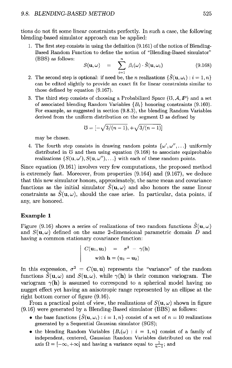
1.
The first
step
consists
in
using
the
definition
(9.161)
of the
notion
of
Blending-
Based Random Function
to
define
the
notion
of
"Blending-Based
simulator"
(BBS)
as follows:
2.
The
second step
is
optional:
if
need
be, the n
realizations
{^(u,
uji)
:
i
=
1,
n}
can be
edited slightly
to
provide
an
exact
fit for
linear constraints similar
to
those
defined
by
equation (9.167).
3.
The
third
step
consists
of
choosing
a
Probabilized Space
(15,
A,
IP)
and a set
of
associated blending Random Variables
{Bi}
honoring constraints (9.160).
For
example,
as
suggested
in
section
(9.8.3),
the
blending Random Variables
derived
from
the
uniform
distribution
on the
segment
13
as
defined
by
may
be
chosen.
4.
The
fourth
step consists
in
drawing random points
{u/,u/',.--}
uniformly
distributed
in
13
and
then using equation (9.168)
to
associate equiprobable
realizations
(5
r
(u,
u/),
S
r
(u,o;"),...}
with each
of
these random points.
Since
equation (9.161) involves very
few
computations,
the
proposed method
is
extremely
fast.
Moreover,
from
properties
(9.164)
and
(9.167),
we
deduce
that
this
new
simulator honors, approximately,
the
same mean
and
covariance
functions
as the
initial simulator
5(u,u;)
and
also honors
the
same linear
constraints
as
5(u,o;),
should
the
case arise.
In
particular,
data
points,
if
any,
are
honored.
Example
1
Figure (9.16) shows
a
series
of
realizations
of two
random
functions
S(u,uj)
and
S(u,uj)
denned
on the
same
2-dimensional
parametric domain
D and
having
a
common
stationary
covariance
function:
In
this expression,
a
2
=
C(u,
u)
represents
the
"variance"
of the
random
functions
S(u,u)
and
5(u,a;),
while 7(h)
is
their common variogram.
The
variogram
7(h)
is
assumed
to
correspond
to a
spherical model having
no
nugget
effect
yet
having
an
anisotropic range represented
by an
ellipse
at the
right
bottom corner
of
figure (9.16).
From
a
practical point
of
view,
the
realizations
of
S(u,uj]
shown
in figure
(9.16)
were generated
by a
Blending-Based simulator (BBS)
as
follows:
• the
base
functions
{S(u,uJi)
: i =
l,n}
consist
of a set of n
=
10
realizations
generated
by a
Sequential Gaussian simulator
(SGS);
• the
blending Random Variables
{Bi(u)
:
i =
l,n}
consist
of a
family
of
independent, centered, Gaussian Random Variables distributed
on the
real
axis
fi
=
[—00,
+00]
and
having
a
variance equal
to
^y;
and
526
CHAPTER
9.
STOCHASTIC MODELING
• the
ergodic
correction
was
applied
to
improve
the
ergodic
behavior.
It is
relevant
to
note
that
the
equiprobability
of the
realizations
of
5(u,
uj]
derives
from
that
of the
blending Random Variables
{Bi(uj)
:
i =
l,n}.
To
check
how
correctly
the SGS and the BBS
methods generate ergodic
realizations honoring
the
specified variogram,
figure
(9.16)
presents
the
spatial
variograms
of ten
realizations obtained with
the BBS
method (top right cor-
ner)
with
the
spatial
variograms
of the
n
= 10 SGS
realizations
(left
bottom
corner)
used
to
define
the
BBS. These
spatial
variograms have been computed
in
the
direction
u
l
corresponding
to the first
component
of the
parameter
u =
[u
1
,
w
2
]*.
As can be
seen,
the
behavior close
to the
origin,
the
range,
and
the
sill
of the
specified
variogram
are
acceptably honored.
In
practice, each equiprobable realization
S(u,
uij)
is
evaluated
at the
nodes
{uffh}
of a
regular grid
in the
parametric domain. Even
for
grids having
one
million
nodes, such
as the
ones shown
in figure
(9.16),
the
computation time
for
a
realization
of a BBS on a
regular
PC is
very
short.
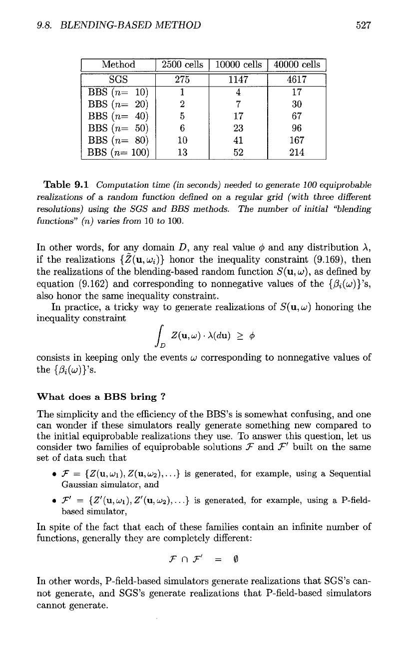
Example
2
A
simple
test
suite
is
presented
in
Table
(9.1)
to
compare
the
performances
of
the BBS
method with
those
of the SGS
method.
In
this
test
suite:
• the
random
function
<S'(u,
o>)
to be
simulated
is
evaluated
at the
nodes
of a 2D
square
grid
and is
assumed
to
have
an
isotropic
spherical
covariance
function
with
a
range
equal
to
one-third
of the
grid
size;
• for
both
methods,
100
(unconstrained)
simulations
are
computed
for
three
different
grid
resolutions
(50 x 50, 100 x
100,
and 200 x 200
cells);
• for the BBS
method,
six
different
values
of the
number
n of
initial
solutions
are
tested
to
evaluate
the
impact
of
this
parameter
on the
computation
time;
• for
each
combination
of
parameters
of the
test
suite,
the
total
computation
time
on an
MIPS
R4400
(200
MHZ)
processor
is
reported
in
Table
(9.1).
As
can be
seen
in
Table
(9.1),
when compared with
the SGS
method
and all
things being equal,
the BBS
method computation time
is at
least
one
order
of
magnitude lower than
that
for the SGS
method. This remarkable computation
speed derives
from
the
simplicity
of
equation (9.162) which involves only
n
multiplications
and n
additions
for
evaluating
a
value
S(ukh,ajj)
at
each node
u
k
h-
9.8.6
Honoring
inequality
constraints
It can
easily
be
checked
that,
if the
inequality constraints
are
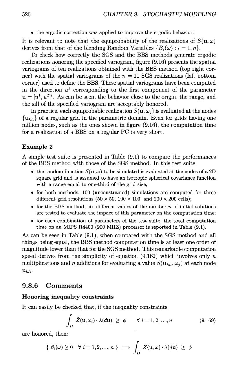
honored, then:
9.8.
BLENDING-BASED
METHOD
527
Table
9.1
Computation
time
(in
seconds)
needed
to
generate
100
equiprobable
realizations
of a
random
function
defined
on a
regular
grid
(with
three
different
resolutions)
using
the SGS and BBS
methods.
The
number
of
initial
"blending
functions"
(n)
varies
from
10 to
100.
In
other words,
for any
domain
Z),
any
real value
0 and any
distribution
A,
if
the
realizations
{Z(u,uJi}}
honor
the
inequality
constraint
(9.169), then
the
realizations
of the
blending-based
random
function
S(u,
u>),
as
defined
by
equation
(9.162)
and
corresponding
to
nonnegative values
of the
{/?j(cj)}'s,
also
honor
the
same inequality constraint.
In
practice,
a
tricky
way to
generate realizations
of
S(u,
oj)
honoring
the
inequality
constraint
consists
in
keeping only
the
events
cu
corresponding
to
nonnegative values
of
the
{AHJ's.
What
does
a BBS
bring
?
The
simplicity
and the
efficiency
of the
BBS's
is
somewhat
confusing,
and one
can
wonder
if
these simulators really generate something
new
compared
to
the
initial equiprobable realizations they use.
To
answer
this
question,
let us
consider
two
families
of
equiprobable solutions
T
and
T'
built
on the
same
set of
data
such
that
•
f
=
(Z(u,u;i),
Z(u,
^2),...}
is
generated,
for
example,
using
a
Sequential
Gaussian
simulator,
and
•
F'
=
{Z'(u,
cui),
Z'(u,
tc>2),
• • •} is
generated,
for
example,
using
a
P-field-
based
simulator,
In
spite
of the
fact
that
each
of
these
families
contain
an
infinite
number
of
functions,
generally they
are
completely
different:
In
other words,
P-field-based
simulators generate realizations
that
SGS's can-
not
generate,
and
SGS's generate realizations
that
P-field-based simulators
cannot generate.
Method
SGS
BBS (n= 10)
BBS (n= 20)
BBS (n= 40)
BBS (n= 50)
BBS (n= 80)
BBS
(n=
100)
2500
cells
275
1
2
5
6
10
13
10000
cells
1147
4
7
17
23
41
52
40000
cells
4617
17
30
67
96
167
214
