Jean-Laurent Mallet. Geomodeling
Подождите немного. Документ загружается.

CHAPTER
1.
DISCRETE MODELING
FOR
NATURAL OBJECTS
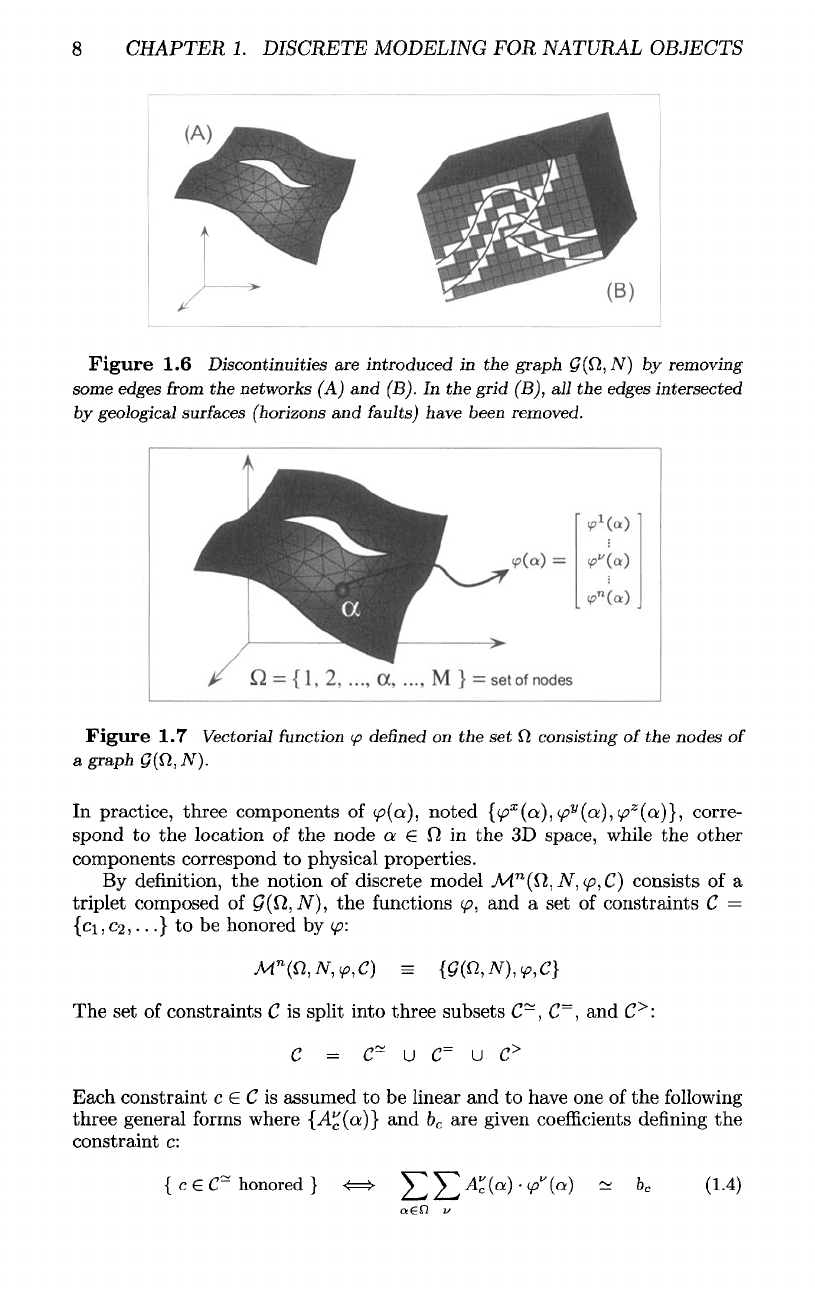
Figure
1.6
Discontinuities
are
introduced
in the
graph
G(Q,N)
by
removing
some
edges
from
the
networks
(A) and
(B).
In the
grid (B),
all the
edges
intersected
by
geological
surfaces
(horizons
and
faults) have been removed.
Figure
1.7
Vectorial function
y>
denned
on the set
0,
consisting
of the
nodes
of
a
graph
g(£l,N).
In
practice, three components
of
(p(ot),
noted
{(p
x
(a),
ip
y
(a),
tp
z
(a)},
corre-
spond
to the
location
of the
node
a
€
O
in the 3D
space, while
the
other
components correspond
to
physical properties.
By
definition,
the
notion
of
discrete model
.M
n
(f2,
N,
<f>,C)
consists
of a
triplet composed
of
Q(Q,N),
the
functions
</?,
and a set of
constraints
C =
{GI,
02,...}
to be
honored
by
(p:
The set of
constraints
C is
split into three subsets
C~,
C
=
,
and
C
>
:
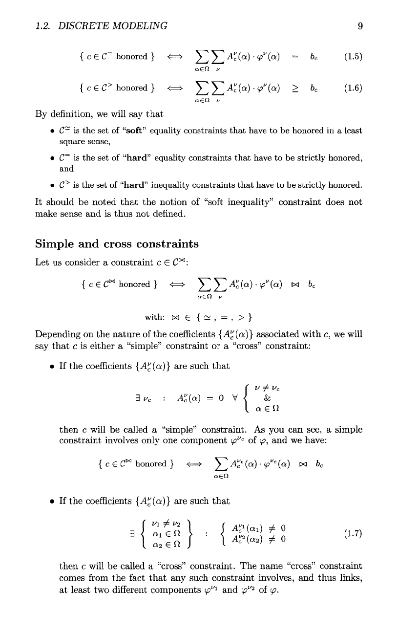
Each constraint
c
e
C is
assumed
to be
linear
and to
have
one of the
following
three general
forms
where
{^(a)}
and
b
c
are
given
coefficients
denning
the
constraint
c:
8
1.2.
DISCRETE MODELING
9
By
definition,
we
will
say
that
•
C~
is the set of
"soft" equality constraints
that
have
to be
honored
in a
least
square sense,
•
C
=
is the set of
"hard" equality constraints
that
have
to be
strictly honored,
and
•
C
>
is the set of
"hard" inequality constraints
that
have
to be
strictly honored.
It
should
be
noted
that
the
notion
of
"soft
inequality" constraint does
not
make sense
and is
thus
not
defined.
Simple
and
cross constraints
Let us
consider
a
constraint
c E
C^:
Depending
on the
nature
of the
coefficients
{A"(a)}
associated
with
c, we
will
say
that
c is
either
a
"simple" constraint
or a
"cross" constraint:
• If the
coefficients
{^(a)}
are
such
that
then
c
will
be
called
a
"simple" constraint.
As you can
see,
a
simple
constraint involves only
one
component
tp
Vc
of
</?,
and we
have:
• If the
coefficients
{A"(a}}
are
such
that
then
c
will
be
called
a
"cross"
constraint.
The
name "cross"
constraint
comes
from
the
fact
that
any
such constraint involves,
and
thus links,
at
least
two
different
components
c^"
1
and
(p
1
"
2
of
(p.
10
CHAPTER
1.
DISCRETE MODELING
FOR
NATURAL OBJECTS
Examples
of
constraints
In
practice,
the
coefficients
{^(CK)}
and
b
c
are
determined
as
functions
of the
available
data;
for
example:
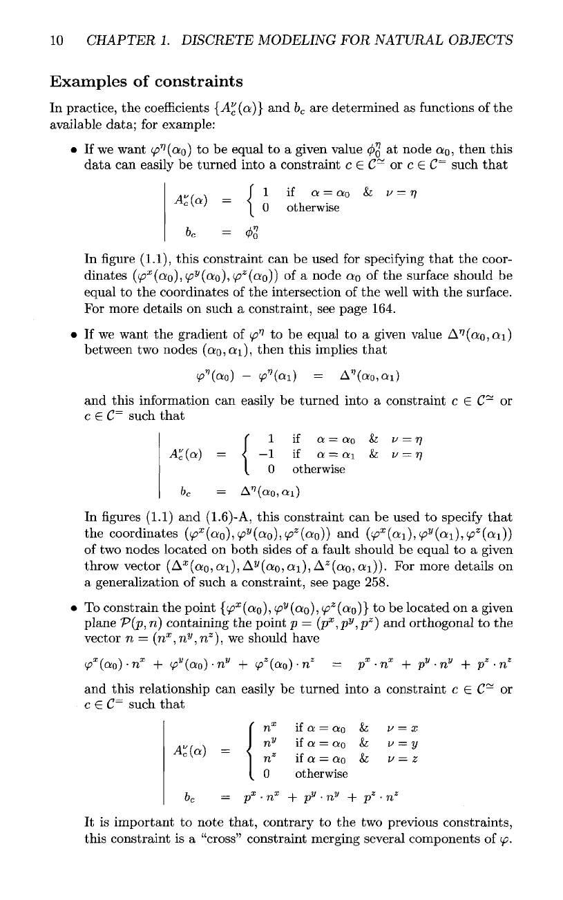
If If we want ^(OLQ) to be equal to a given value $} at node a
0
>
then this
data
can
easily
be
turned into
a
constraint
c 6
C~
or c
G
C
=
such
that
In
figure
(1.1),
this constraint
can be
used
for
specifying
that
the
coor-
dinates
((/?
X
(Q:O),
(p
y
(oto),
(p
z
(oio)}
of a
node
ao
of the
surface should
be
equal
to the
coordinates
of the
intersection
of the
well
with
the
surface.
For
more details
on
such
a
constraint,
see
page
164.
If we
want
the
gradient
of
(fP
to be
equal
to a
given value
A
77
(ceo
,0:1)
between
two
nodes
(ao,a:i),
then this implies
that
p"(ao)
-
¥>"(ai)
=
A"(a
0
,ai)
and
this information
can
easily
be
turned into
a
constraint
c 6
C~
or
c
e
C
=
such
that
In
figures
(1.1)
and
(1.6)-A, this constraint
can be
used
to
specify
that
the
coordinates
(p
x
(a
0
),
tp
y
(a
0
),
ip
z
(o>
0
))
and
(p
x
(ai),
(p
y
(ai),
ip
z
(ai})
of
two
nodes located
on
both sides
of a
fault
should
be
equal
to a
given
throw
vector
(A
x
(ao,ai),
A
y
(a
0
,ai),
A^o^cei))-
For
more details
on
a
generalization
of
such
a
constraint,
see
page 258.
To
constrain
the
point
{(f>
x
(UQ),
(p
y
(a
Q
},
(p
z
(ao)}
to be
located
on a
given
plane
P(p,
ri)
containing
the
point
p =
(p
x
,p
y
,p
z
)
and
orthogonal
to the
vector
n =
(n
x
,n
y
,n
z
),
we
should have
(
and
this
relationship
can
easily
be
turned into
a
constraint
c G
C~
or
c G
C~
such
that
It is
important
to
note
that,
contrary
to the two
previous constraints,
this constraint
is a
"cross" constraint merging several components
of
(p.
1.2.
DISCRETE
MODELING
11
and
this
relationship
can
easily
be
turned into
a
constraint
c
e
C~
or
c G
C~
such
that
In
this case,
the
total
number
of
constraints
attached
to the
node
Q.Q
is
then
(In
+ 1). For
more
details
on the use and
implementation
of
such
constraints,
see
page 540.
• Let
|f2|
be the
number
of
elements
of the set
Jl.
If we
want
to
specify
that
the
average value
of a
function
</?"
over
£7
is
equal
to a
given value
</?",
then
we
should have
and
this
relationship
can
easily
be
turned into
a
constraint
c
G
C~
or
c
G
C
=
such
that
For
more
details
on
such
a
constraint,
see
page 548.
• If
(p
11
is the
pressure
of
water
(or
oil)
in a
given layer, then
^
has to re-
spect
the
diffusion
equation. Such
an
equation
can
always
be
discretized
with
a finite
difference
or finite
element method
(Aziz
and
Settari
[10])
In figure
(1.1),
this
constraint
can be
used
for
specifying
that
a
node
ao
should
be
located
in a
given tangent plane.
For
more details
on
such
a
constraint,
see
page 265.
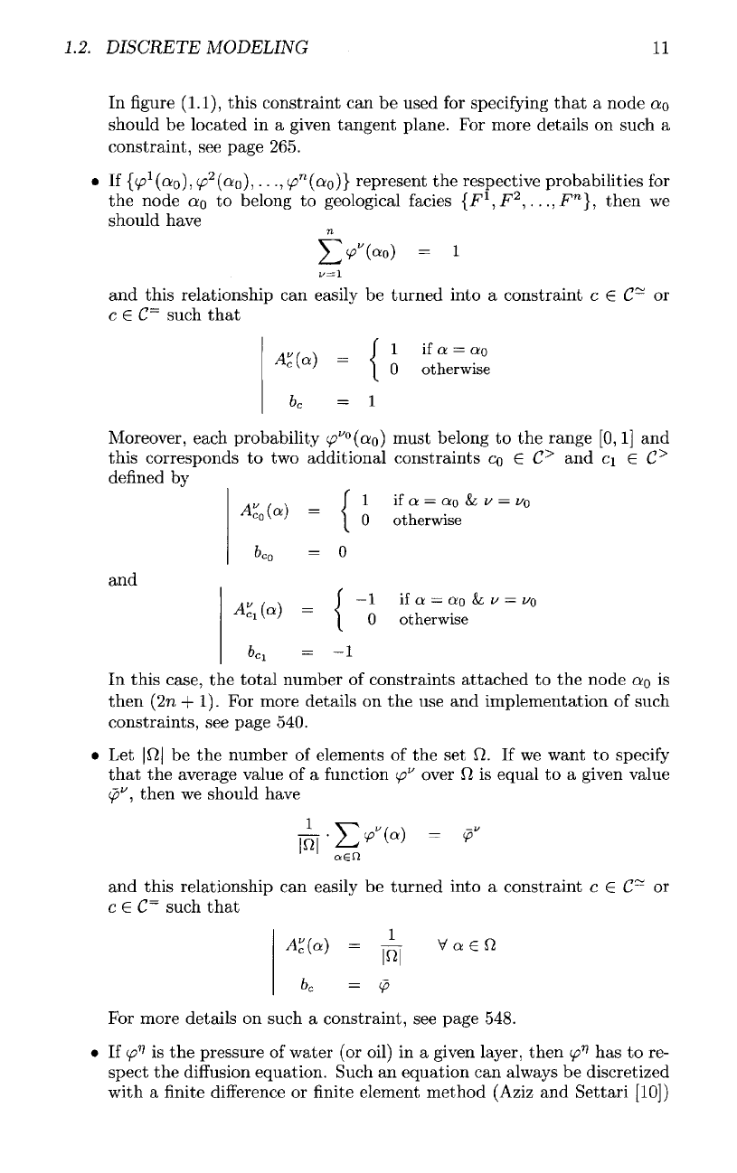
• If
{v?
1
(a
0
),
V^^o),
• •
-,
<^
n
(o!o)}
represent
the
respective probabilities
for
the
node
a
0
to
belong
to
geological
facies
{F
l
,F
2
,...,
F
n
},
then
we
should have
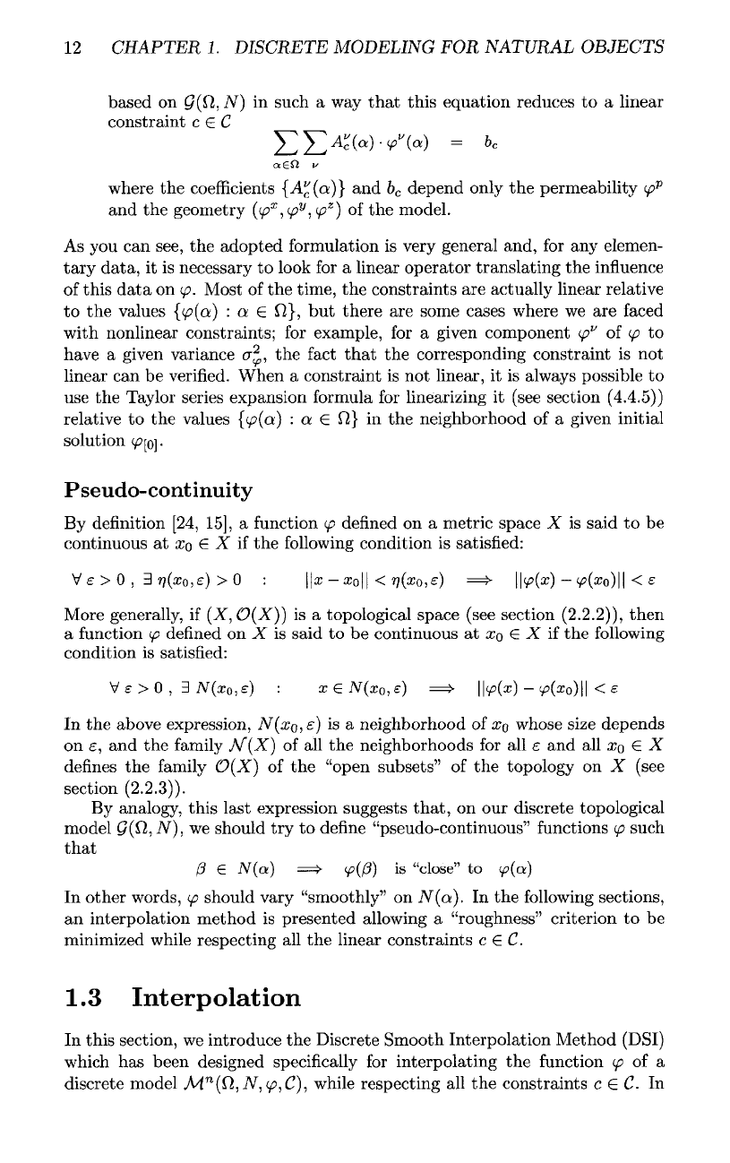
n.
Moreover,
each probability
<^"°(a;o)
must belong
to the
range
[0,1]
and
this corresponds
to two
additional constraints
CQ
G
C
>
and c\ G
C
>
defined
by
12
CHAPTER
1.
DISCRETE MODELING
FOR
NATURAL OBJECTS
based
on
(/(£),
JV)
in
such
a way
that
this equation reduces
to a
linear
constraint
c
(E
C
where
the
coefficients
{^(a)}
and
b
c
depend only
the
permeability
(p
p
and the
geometry
((p
x
,
(p
y
,(p
z
)
of the
model.
As
you can
see,
the
adopted
formulation
is
very general and,
for any
elemen-
tary
data,
it is
necessary
to
look
for a
linear operator translating
the
influence
of
this
data
on
(p.
Most
of the
time,
the
constraints
are
actually linear relative
to the
values
{<p(a)
'. a G
0},
but
there
are
some cases where
we are
faced
with
nonlinear constraints;
for
example,
for a
given component
(p
v
of
</?
to
have
a
given variance
cr^,,
the
fact
that
the
corresponding constraint
is not
linear
can be
verified.
When
a
constraint
is not
linear,
it is
always possible
to
use the
Taylor series expansion
formula
for
linearizing
it
(see section
(4.4.5))
relative
to the
values
{(p(a)
:
a G
£7}
in the
neighborhood
of a
given initial
solution
</?[o]
•
Pseudo-continuity
By
definition
[24, 15],
a
function
</?
defined
on a
metric space
X is
said
to be
continuous
at
XQ
6 X if the
following
condition
is
satisfied:
More
generally,
if
(X,O(X))
is a
topological space (see section
(2.2.2)),
then
a
function
(p
defined
on X is
said
to be
continuous
at
XQ
£ X if the
following
condition
is
satisfied:
In the
above expression,
N(XQ,£)
is a
neighborhood
of
XQ
whose size
depends
on
£,
and the
family
N(X)
of all the
neighborhoods
for all
e
and all
XQ
G X
defines
the
family
O(X]
of the
"open
subsets"
of the
topology
on X
(see
section
(2.2.3)).
By
analogy, this last expression suggests
that,
on our
discrete topological
model
C?(fJ,
N),
we
should
try to
define
"pseudo-continuous"
functions
(p
such
that
In
other words,
(p
should vary "smoothly"
on
N(a).
In the
following
sections,
an
interpolation method
is
presented allowing
a
"roughness" criterion
to be
minimized
while respecting
all the
linear constraints
c G
C.
1.3
Interpolation
In
this section,
we
introduce
the
Discrete Smooth Interpolation Method
(DSI)
which
has
been designed specifically
for
interpolating
the
function
(p of a
discrete model
M.
n
(£l,
N,
</?,£),
while respecting
all the
constraints
c G C. In
INTE
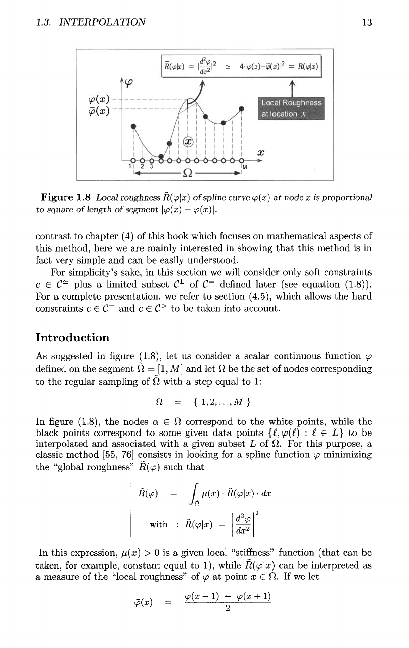
Figure
1.8
Local roughness
R(ip
x)
of
spline curve
<p(x)
at
node
x is
proportional
to
square
of
length
of
segment
|v?(x)
—
<f>(x)\.
contrast
to
chapter
(4) of
this book which
focuses
on
mathematical
aspects
of
this method, here
we are
mainly interested
in
showing
that
this
method
is in
fact
very simple
and can be
easily understood.
For
simplicity's sake,
in
this section
we
will
consider only
soft
constraints
c
G
C~
plus
a
limited subset
C
L
of
C^
defined
later (see equation
(1.8)).
For a
complete presentation,
we
refer
to
section
(4.5),
which allows
the
hard
constraints
c
(E
C=
and c 6
£>
to be
taken
into account.
Introduction
As
suggested
in figure
(1.8),
let us
consider
a
scalar continuous
function
(p
defined
on the
segment
17
=
[1,
M]
and let 17 be the set of
nodes corresponding
to the
regular sampling
of 17
with
a
step
equal
to
1:
In
figure
(1.8),
the
nodes
a € 17
correspond
to the
white points, while
the
black
points correspond
to
some given
data
points
{£,
(p(l)
:
I
€ L} to be
interpolated
and
associated with
a
given subset
L of 17. For
this purpose,
a
classic method [55,
76]
consists
in
looking
for a
spline
function
ip
minimizing
the
"global roughness"
R((p]
such
that
In
this expression,
[i(x)
> 0 is a
given local
"stiffness"
function
(that
can be
taken,
for
example, constant equal
to 1),
while
R((p\x)
can be
interpreted
as
a
measure
of the
"local roughness"
of
(p
at
point
x € 17. If we let
INTERPOLATION
13
14
CHAPTER
1.
DISCRETE MODELING
FOR
NATURAL OBJECTS
then,
as
suggested
in figure
(1.8),
we can
verify
that
a finite
difference
ap-
proximation
of
d?(p/dx
2
is
such
that
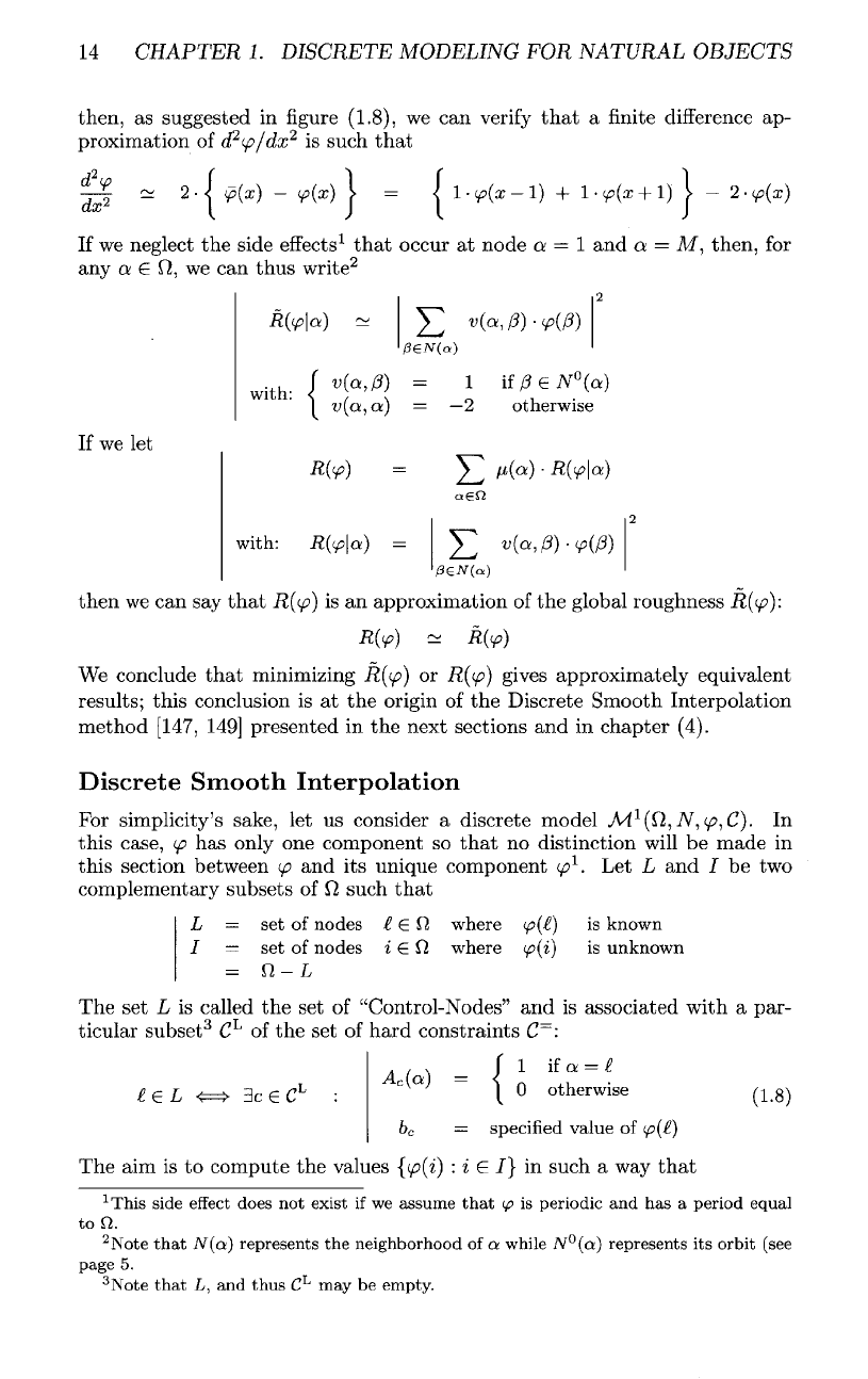
If
we
neglect
the
side
effects
1
that
occur
at
node
a
=
1 and a =
M,
then,
for
any
a
e
fJ,
we can
thus
write
2
then
we can say
that
R((p)
is an
approximation
of the
global roughness
R((p):
We
conclude
that
minimizing
R((p]
or
R((p)
gives approximately equivalent
results; this conclusion
is at the
origin
of the
Discrete Smooth Interpolation
method [147, 149] presented
in the
next sections
and in
chapter (4).
Discrete
Smooth
Interpolation
For
simplicity's sake,
let us
consider
a
discrete model
A
/
(
1
(O,
TV,
</?,
C).
In
this case,
(p
has
only
one
component
so
that
no
distinction
will
be
made
in
this section between
(p
and its
unique component
<p
l
.
Let L and I be two
complementary
subsets
of
f2
such
that
The set L is
called
the set of
"Control-Nodes"
and is
associated with
a
par-
ticular
subset
3
C
L
of the set of
hard constraints
C
=
:
lr
This
side
effect
does
not
exist
if we
assume
that
(p
is
periodic
and has a
period equal
to
n.
2
Note
that
N(a)
represents
the
neighborhood
of a
while
JV°(a)
represents
its
orbit (see
page
5.
3
Note
that
L, and
thus
C
L
may be
empty.
Tje
aim is to compute the values in such a way that
1.3.
INTERPOLATION
15
• the
resulting function
</?
be "as
smooth
as
possible"
on
C/(f7,
TV),
• the
"control values"
{</?(•£)
:
£
G
I/}
be
strictly honored,
and
•
each
of the
constraints
4
c 6
C~
be
respected
"as
much
as
possible."
For
this
purpose,
we
propose
to
measure
the
local roughness
R((p
a]
of
(p
in
the
neighborhood
of
each node
a
G
0
and the
degree
of
violation
p(p\c)
of
each constraint
c 6
C~
by
(p
as
follows:
In
this definition
of the
local roughness
jR(<^|o;),
the
{v(a,
/3)}'s
are
arbitrarily
given
coefficients
(e.g.,
see
page 149)
and the
Discrete Smooth Interpolation
method
(DSI)
proposes
to
look
for a
function
ip
minimizing
the
following
"generalized
roughness" criterion
R*((p}:
In
this criterion:
•
(i(a)
> 0 is a
given positive "stiffness" function modulating
the
importance
of
the
local roughness
R(<p\a)
at
node
a,
•
{ta
c
}
are
positive "certainty factors" weighting
the
importance
of
constraints
relative
to
each other,
and
• (0 •
TJJ)
is a
term
to be
determined
to
balance
the
order
of
magnitude
of
N
w
c
•
p(f\c)
relative
to
N
V>(oi)
•
R((p\a).
esc-
aen
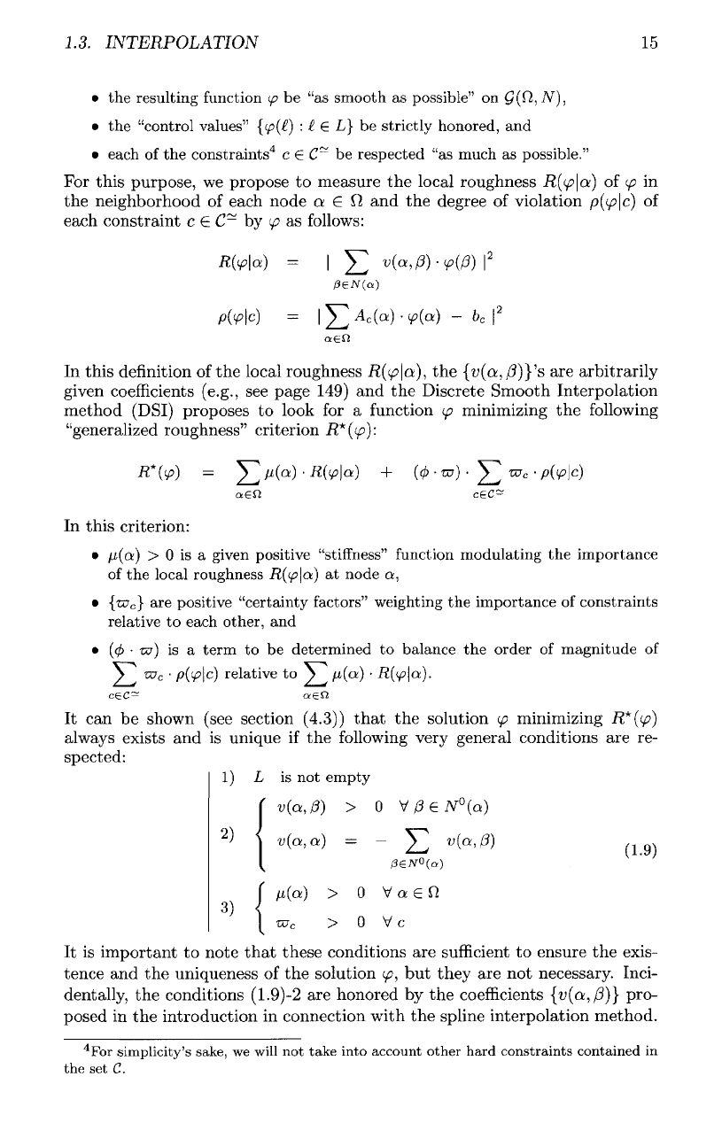
It can be
shown (see section
(4.3))
that
the
solution
(p
minimizing
R*(<p}
always exists
and is
unique
if the
following
very general conditions
are re-
spected:
It is
important
to
note
that
these conditions
are
sufficient
to
ensure
the
exis-
tence
and the
uniqueness
of the
solution
</?,
but
they
are not
necessary. Inci-
dentally,
the
conditions (1.9)-2
are
honored
by the
coefficients
{v(a,P}}
pro-
posed
in the
introduction
in
connection with
the
spline interpolation method.
4
For
simplicity's
sake,
we
will
not
take
into
account
other
hard
constraints
contained
in
the set
C.
1)
L is not empty
2)
3)
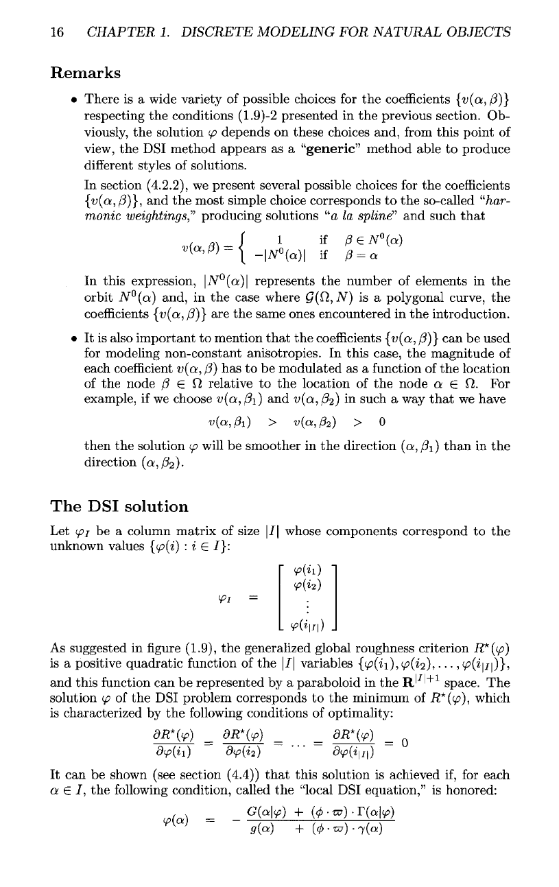
15
16
CHAPTER
1.
DISCRETE MODELING
FOR
NATURAL OBJECTS
Remarks
•
There
is a
wide variety
of
possible choices
for the
coefficients
{v(a,(3)}
respecting
the
conditions
(1.9)-2
presented
in the
previous section.
Ob-
viously,
the
solution
</?
depends
on
these choices and,
from
this point
of
view,
the
DSI
method appears
as a
"generic" method able
to
produce
different
styles
of
solutions.
In
section
(4.2.2),
we
present several possible choices
for the
coefficients
{v(a,
/?)},
and the
most simple choice corresponds
to the
so-called "har-
monic weightings" producing solutions
"a la
spline"
and
such
that
In
this expression,
\N°(a)
represents
the
number
of
elements
in the
orbit
7V°(o;)
and,
in the
case where
C?(Q,7V")
is a
polygonal curve,
the
coefficients
{v(a,
(3)}
are the
same ones encountered
in the
introduction.
It is
also important
to
mention
that
the
coefficients
{v(a,
(3)}
can be
used
for
modeling non-constant anisotropies.
In
this
case,
the
magnitude
of
each
coefficient
v(a,
(3)
has to be
modulated
as a
function
of the
location
of
the
node
f3
6 0
relative
to the
location
of the
node
a 6 fi. For
example,
if we
choose
v(a,{3i)
and
v(a,
fa) in
such
a way
that
we
have
then
the
solution
(p
will
be
smoother
in the
direction
(a,
@i)
than
in the
direction
(a,
fa).
The DSI
solution
Let
(/?/
be a
column matrix
of
size
/|
whose components correspond
to the
unknown
values
{<p(i)
: i € /}:
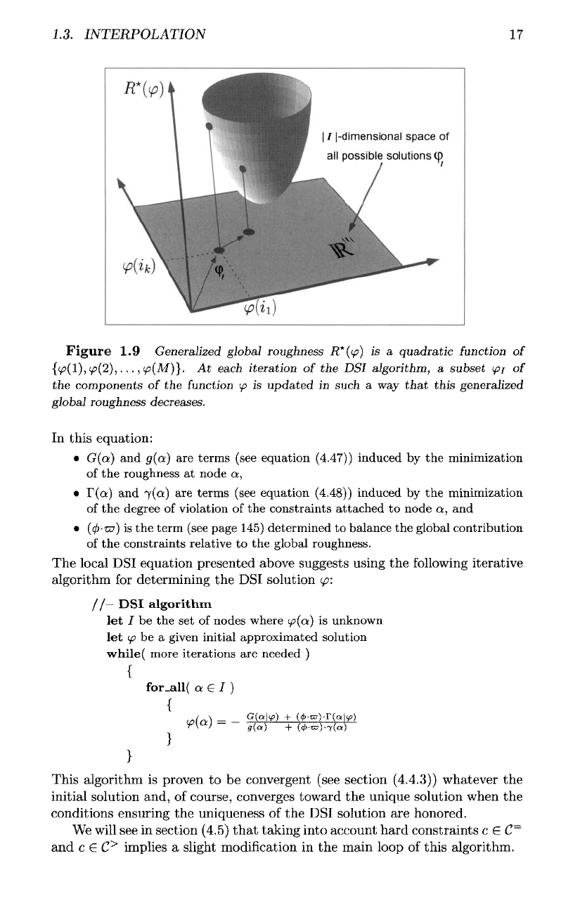
As
suggested
in figure
(1.9),
the
generalized global roughness criterion
R*(^>)
is a
positive quadratic
function
of the |/|
variables
{(p(ii),(p(i
2
),...,
<f>(i\i\)},
and
this
function
can be
represented
by a
paraboloid
in the R'
'
+1
space.
The
solution
(p
of the DSI
problem corresponds
to the
minimum
of
R*(<p),
which
is
characterized
by the
following
conditions
of
optimality:
It can be
shown (see section
(4.4))
that
this solution
is
achieved
if, for
each
a G /, the
following
condition, called
the
"local
DSI
equation,"
is
honored:
1.3.
INTERPOLATION
17
Figure
1.9
Generalized global roughness
R*((p)
is a
quadratic function
of
{
¥?(!),
y?(2),...,
y>(M)}.
At
each
iteration
of the
DSI
algorithm,
a
subset
(pi
of
the
components
of the
function
(p
is
updated
in
such
a way
that
this generalized
global
roughness decreases.
In
this equation:
•
G(o)
and
g(ci)
are
terms
(see
equation
(4.47))
induced
by the
minimization
of
the
roughness
at
node
a,
•
r(a)
and
7(0;)
are
terms (see
equation
(4.48))
induced
by the
minimization
of
the
degree
of
violation
of the
constraints attached
to
node
a, and
•
(</>••£?)
is the
term
(see
page
145)
determined
to
balance
the
global contribution
of
the
constraints relative
to the
global roughness.
The
local
DSI
equation presented above suggests using
the following
iterative
algorithm
for
determining
the DSI
solution
(p:
/I-
DSI
algorithm
let
/
be the set of
nodes where
tp(
a
)
i
s
unknown
let
(p
be a
given initial approximated solution
while
(
more iterations
are
needed
)
This algorithm
is
proven
to be
convergent (see section
(4.4.3))
whatever
the
initial solution and,
of
course, converges toward
the
unique solution when
the
conditions ensuring
the
uniqueness
of the DSI
solution
are
honored.
We
will
see in
section (4.5)
that
taking into account
hard
constraints
c G
C~
and c 6
C
>
implies
a
slight
modification
in the
main loop
of
this algorithm.
