Jacques I. Mathematics for Economics and Business

Подождите немного. Документ загружается.

Appendix 1 • Differentiation from First Principles

590

Practice Problems

2 Use ﬁrst principles to differentiate each of the following functions

(a)

y = 4x

− 9x + 1 (b) y =

3 (a) By writing (a + b)

= (a + b)(a + b)

show that

(a + b)

= a

+ 3a

b + 3ab

+ b

(b) Use the result of part (a) to prove that the cube function, x

, differentiates to 3x

MFE_Z01.qxd 16/12/2005 10:50 Page 590

The idea of implicit differentiation was ﬁrst introduced in Section 5.1 (page 354) in the context

of partial differentiation. It is possible to approach this topic via ordinary differentiation.

Indeed, it can be regarded as nothing more than a simple application of the chain rule.

Appendix 2

Implicit

Differentiation

Example

Use implicit differentiation to ﬁnd the value of on the curve

(a) y

− 2x

= 25 at the point (−2,3)

(b) ln y + 3y − x

= 2 at the point (1,1)

Solution

(a) The ﬁrst thing to do is to differentiate both sides of y

− 2x

= 25 with respect to x.

To differentiate the term (y)

with respect to x, you ﬁrst differentiate the outer ‘square’ function to get

2y and then multiply by the derivative of inner function, y, with respect to x, which is dy/dx. Hence

( y

) = 2y

The remaining terms are more easily dealt with:

(2x

) = 6x

and (25) = 0

Collecting these results together gives

2y − 6x

= 0

so that



MFE_Z01.qxd 16/12/2005 10:50 Page 591

Finally, substituting x =−2, y = 3, gives

==4

(b) To differentiate the term ln(y) with respect to x we use the chain rule. The outer log function goes to

and the inner ‘y’ function differentiates to . Hence

(ln( y)) =×

Again the other terms are more straightforward:

(3y) = 3, (x

) = 2x and (2) = 0

Differentiating both sides of ln y + 3y − x

= 2 with respect to x gives:

+ 3 − 2x = 0

To make dy/dx the subject of this equation, ﬁrst multiply both sides by y to get

+ 3 y − 2xy = 0

(1 + 3y) = 2xy (add 2xy to both sides and then factorize the left-hand side)

= (divide both sides by 1 + 3y)

Finally, substituting, x = 1, y = 1 gives

2(1)(1)

1 + 3(1)

2xy

1 + 3y

3(−2)

Appendix 2 • Implicit Differentiation

592

Practice Problem

1 (a) Verify that the point (1, 2) lies on the curve 2x

+ 3y

= 14.

(b) By differentiating both sides of 2x

+ 3y

= 14 with respect to x, show that

=−

and hence ﬁnd the gradient of the curve at (1,2).

In the previous example each of the terms involves just one of the letters x or y. It is pos-

sible to handle more complicated terms that involve both letters. For example, to differentiate

the term ‘xy’ with respect to x, we use the product rule, which gives

(xy) = x + 1 × y = x + y

This is illustrated in the following example.

MFE_Z01.qxd 16/12/2005 10:50 Page 592

Appendix 2 • Implicit Differentiation

593

Practice Problem

2 By differentiating both sides of the following with respect to x, ﬁnd expressions for in terms of

x and y.

(a)

+ y

= 16

(b) 3y

+ 4x

+ 2x = 2

+ 2e

= 1

(d) ye

= xy + y

(e) x

+ 2xy

− 3y = 10

(f) ln (x + y) =−x

Example

Find an expression for in terms of x and y for

+ 3y

− xy = 11

Solution

Differentiating both sides with respect to x gives

2x + 6y − x + y = 0 (chain and product rules)

2x + 6y − x − y = 0 (multiply out brackets)

2x − y + (6y − x) = 0 (collect terms)

= (make the subject)

y − 2x

6y − x

MFE_Z01.qxd 16/12/2005 10:50 Page 593

In this appendix we describe what a Hessian is, and how it can be used to classify the station-

ary points of an unconstrained optimization problem. In Section 5.4 (page 391) the conditions

for a function f(x, y) to have a minimum were stated as:

> 0, f

> 0 and f

− f

> 0

where all of the partial derivatives are evaluated at a stationary point, (a, b).

It turns out that the second condition, f

> 0, is actually redundant. If the ﬁrst and third

conditions are met then the second one is automatically true. To see this notice that

− f

> 0

is the same as f

> f

. The right-hand side is non-negative (being a square term) and so

> 0

The only way that the product of two numbers is positive is when they are either both positive

or both negative. Consequently, when f

> 0, say, the other factor f

will also be positive.

Similarly, for a maximum point f

< 0, which forces the condition f

< 0.

The two conditions for a minimum point, f

> 0 and f

− f

> 0 can be expressed more

succinctly in matrix notation.

The 2 × 2 matrix, H = (where f

= f

) made from second-order partial derivatives

is called a Hessian matrix and has determinant

= f

− f

so the conditions for a minimum are:

(1) the number in the top left-hand corner of H (called the ﬁrst principal minor) is positive

(2) the determinant of H (called the second principal minor) is positive.

For a maximum, the ﬁrst principal minor is negative and the second principal minor is

positive.

Appendix 3

Hessians

MFE_Z01.qxd 16/12/2005 10:50 Page 594

Appendix 3 • Hessians

595

Example

Use Hessians to classify the stationary point of the function

π=50Q

− 2Q

+ 95Q

− 4Q

− 3Q

Solution

This proﬁt function, considered in Practice Problem 2 in Section 5.4 (page 394), has a stationary point at

= 5, Q

= 10. The second-order partial derivatives are

=−4, =−8 and =−3

so the Hessian matrix is

H =

The ﬁrst principal minor −4 < 0.

The second principal minor (−4)(−8) − (−3)

= 23 > 0.

Hence the stationary point is a maximum.

−4 −3

−3 −8

∂

∂Q

∂

∂Q

∂

∂Q

Practice Problems

1 The function

z = x

+ y

− 2x − 4y + 15

has a stationary point at (1,2). Write down the associated Hessian matrix and hence determine the

nature of this point.

[This surface was previously sketched using Maple in Practice Problem 10(a) in Section 5.4 at page 399.]

2 The proﬁt function

π=1000Q

+ 800Q

− 2Q

− Q

has a stationary point at Q

= 100, Q

= 300.

Use Hessians to show that this is a maximum.

[This is the worked example on page 392 of Section 5.4.]

3 The proﬁt function

π=16L

1/ 2

+ 24K

1/ 2

− 2L − K

has a stationary point at L = 16, K = 144.

Write down a general expression for the Hessian matrix in terms of L and K, and hence show that

the stationary point is a maximum.

[This is Practice Problem 7 on page 399 of Section 5.4.]

MFE_Z01.qxd 16/12/2005 10:50 Page 595

Matrices can also be used to classify the maximum and minimum points of constrained

optimization problems. In Section 5.6 the Lagrangian function was deﬁned as

g(x, y, λ) = f(x, y) +λ(M −φ(x, y))

Optimum points are found by applying the three ﬁrst-order conditions:

= 0, g

= 0 and g

= 0

To classify as a maximum or minimum we consider the determinant of the 3 × 3 matrix of

second-order derivatives:

If |H

|>0 the optimum point is a maximum, whereas if |H

|<0, the optimum point is a

minimum.

Note that

= M −φ(x, y)

so that

=−φ

, =−φ

and = 0

so H

is given by

This is called a bordered Hessian because it consists of the usual 2 × 2 Hessian

‘bordered’ by a row and column of ﬁrst-order derivatives, −φ

, −φ

and 0.

−φ

∂

∂λ

∂

∂y∂λ

∂

∂x∂λ

∂g

∂λ

xλ

yλ

x λ

y λ

λλ

Appendix 3 • Hessians

596

Example

Use the bordered Hessian to classify the optimal point when the objective function

U = x

1/ 2

+ x

1/ 2

is subject to the budgetary constraint

+ P

= M

Solution

The optimal point has already been found in Practice Problem 3 of Section 5.6 (page 418). The ﬁrst-order

conditions

= x

−1/ 2

−λP

= 0, = x

−1/2

−λP

= 0, = M − P

− P

= 0

were seen to have solution

∂g

∂λ

∂g

∂x

∂g

∂x

MFE_Z01.qxd 16/12/2005 10:50 Page 596

= and x

The bordered Hessian is

Expanding along the third row gives

|=−P

− (−P

)

= P

−3/ 2

+ P

−3/ 2

This is positive so the point is a maximum.

−

−3/ 2

−P

0 −P

−

−3/ 2

−P

+ P

)

+ P

)

Appendix 3 • Hessians

597

Practice Problems

4 Use the bordered Hessian to show that the optimal value of the Lagrangian function

g(Q

, Q

, λ) = 40Q

− Q

+ 2Q

+ 20Q

− Q

+λ(15 − Q

− Q

)

is a maximum.

[This is the worked example on page 415 of Section 5.6.]

5 Use the bordered Hessian to classify the optimal value of the Lagrangian function

g(x, y, λ) = 2x

− xy +λ(12 − x − y)

[This is Practice Problem 1 on page 413 of Section 5.6.]

Bordered Hessian matrix A Hessian matrix augmented by an extra row and column

containing partial derivatives formed from the constraint in the method of Lagrange

multipliers.

First principal minor The 1 × 1 determinant in the top left-hand corner of a matrix; the

element a

of a matrix A.

Hessian matrix A matrix whose elements are the second-order partial derivatives of a

given function.

Second principal minor The 2 × 2 determinant in the top left-hand corner of a matrix.

Key Terms

− x

−3/ 2

0 −P

0 − x

−3/ 2

−P

MFE_Z01.qxd 16/12/2005 10:50 Page 597

Getting Started

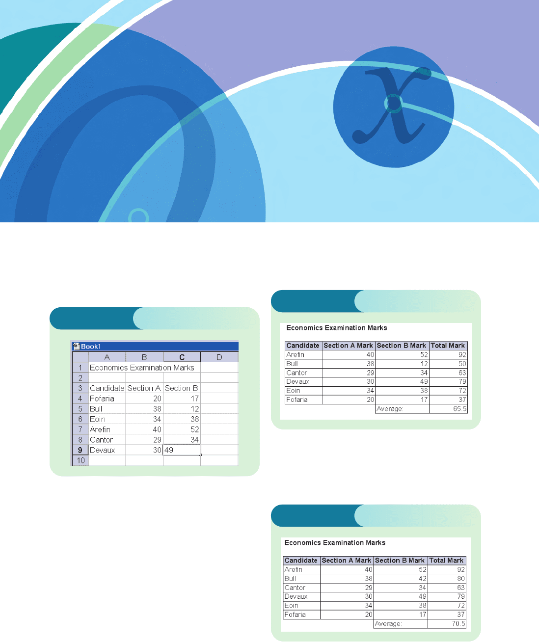
1 (a) This is shown in Figure SI.1.

(e) Just put the cursor over cell C5 and type in the new

mark of 42. Pressing the Enter key causes cells D5

and D10 to be automatically updated. The new

spreadsheet is shown in Figure SI.3.

Solutions to

Problems

Figure SI.1

Figure SI.2

Figure SI.3

(b) Type the heading Total Mark in cell D3.

Type

=B4+C4 into cell D4. Click and drag down

to D9.

Type

=(SUM(D4:D9))/6 in cell D10 and press Enter.

[Note: Excel has lots of built-in functions for

performing standard calculations such as this.

To ﬁnd the average you could just type

=AVERAGE(D4:D9) in cell D10.]

(d) This is shown in Figure SI.2.

MFE_Z02.qxd 16/12/2005 10:51 Page 598

2 (a) 14

(b) 11

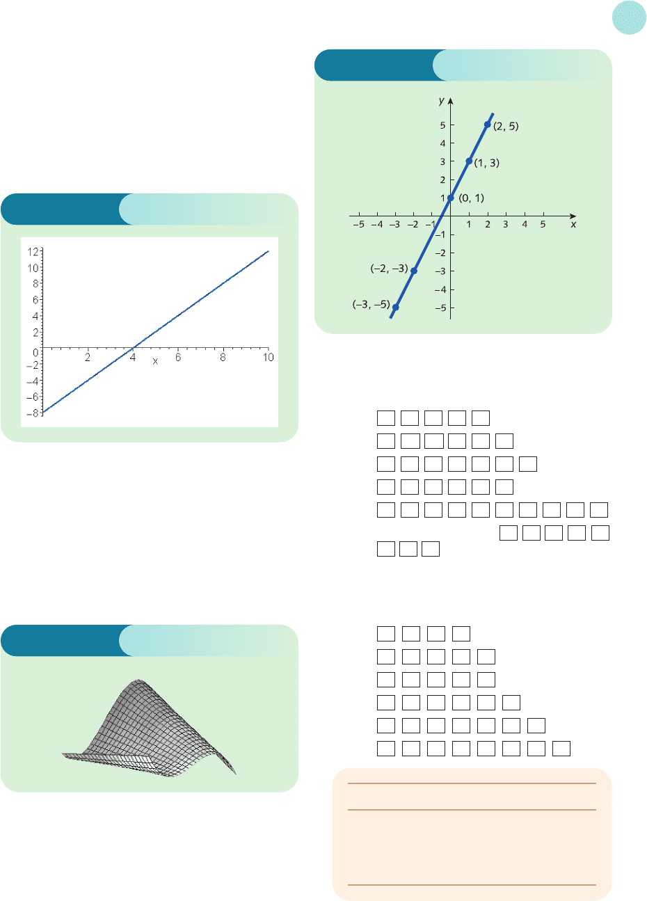
3 (a) 4; is the solution of the equation 2x − 8 = 0.

(b) Figure SI.4 shows the graph of 2x − 8 plotted

between x = 0 and 10.

2 (1) (a) −30; (b) 2; (c) −5;

(d) 5; (e) 36; (f) −1.

(2) The key sequences (working from left to right) are

(a) 5 ×±6 =

(b) ± 1 ×±2 =

(d) ± 5 ÷±1 =

(e) 2 ×±1 ×±3 × 6 =

(f) same as (e) followed by ÷ ± 2 ÷ 3

÷ 6 =

3 (1) (a) −1; (b) −7; (c) 5;

(d) 0; (e) −91; (f ) −5.

(2) The key sequences are

(a) 1 −

2 =

(b) ± 3 − 4 =

(d) ± 1 −±1 =

(e) ± 72− 19=

(f) ± 53−±48=

Solutions to Problems

599

Figure SI.4

Figure SI.5

Chapter 1

Section 1.1

1 From Figure S1.1 note that all ﬁve points lie on a

straight line.

+ 4x + 4; the brackets have been ‘multiplied out’

in the expression (x + 2)

(d) 7x + 4; like terms in the expression 2x + 6 + 5x − 2

have been collected together.

(e) Figure SI.5 shows the three-dimensional graph of

the surface x

− 3x + xy plotted between −2 and 2 in

both the x and y directions.

Figure S1.1

Point Check

(−1, 2) 2(−1) + 3(2) =−2 + 6 = 4 ✓

(−4, 4) 2(−4) + 3(4) =−8 + 12 = 4 ✓

(5, −2) 2(5) + 3(−2) = 10 − 6 = 4 ✓

(2, 0) 2(2) + 3(0) = 4 + 0 = 4 ✓

The graph is sketched in Figure S1.2 (overleaf).

MFE_Z02.qxd 16/12/2005 14:38 Page 599