Jacques I. Mathematics for Economics and Business
Подождите немного. Документ загружается.

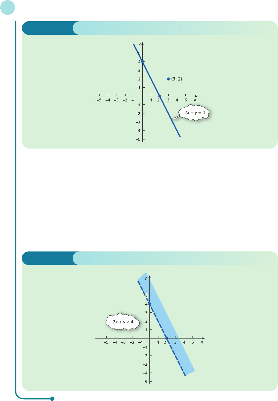
When y = 0 we get
2x = 4
and so x = 4/2 = 2.
The line passes through (0, 4) and (2, 0) and is shown in Figure 8.3. For a test point let us take (3, 2),
which lies above the line. Substituting x = 3 and y = 2 into the expression 2x + y gives
2(3) + 2 = 8
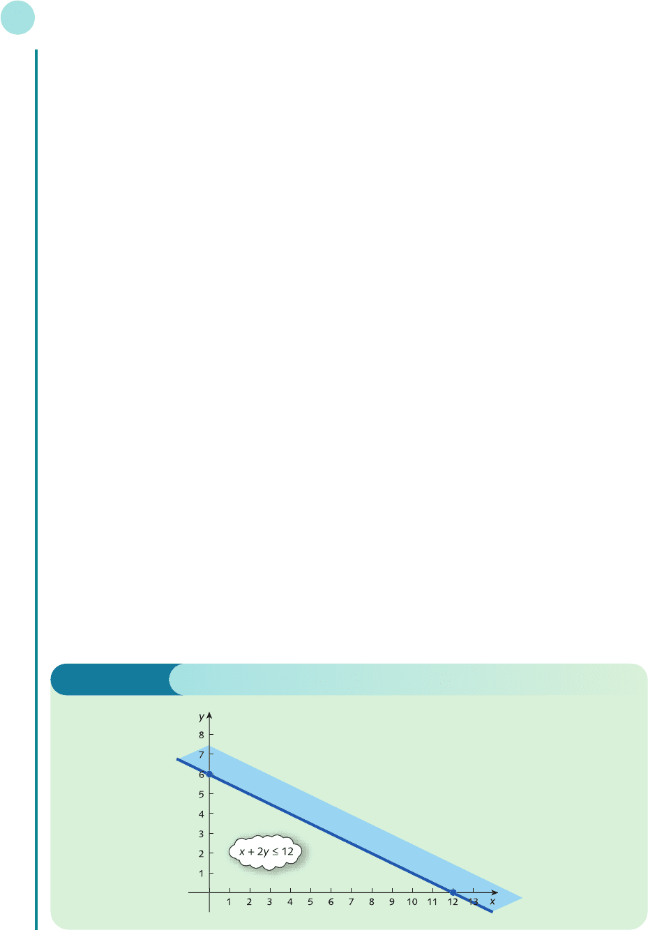
This is not less than 4, so the test point does not satisfy the inequality. It follows that the region of interest
lies below the line. This is illustrated in Figure 8.4. In this example the symbol < is used rather than ≤. Hence
the points on the line itself are not included in the region of interest. We have chosen to indicate this by
using a broken line for the boundary.
Linear Programming
520
Figure 8.3
Figure 8.4
MFE_C08a.qxd 16/12/2005 10:47 Page 520

We now consider the region defined by simultaneous linear inequalities. This is known as a
feasible region. It consists of those points (x, y) which satisfy several inequalities at the same
time. We find it by sketching the regions defined by each inequality in turn. The feasible region
is then the unshaded part of the plane corresponding to the intersection of all of the individual
regions.
8.1 • Graphical solution of linear programming problems
521
Practice Problem
1 Sketch the straight line
−x + 3y = 6
on graph paper. By considering the test point (1, 4) indicate the region
−x + 3y > 6
Example
Sketch the feasible region
x + 2y ≤ 12
−x + y ≤ 3
x ≥ 0
y ≥ 0
Solution
In this problem the easiest inequalities to handle are the last two. These merely indicate that x and y are non-
negative and so we need only consider points in the top right-hand quadrant of the plane, as shown in
Figure 8.5.
Figure 8.5
MFE_C08a.qxd 16/12/2005 10:47 Page 521
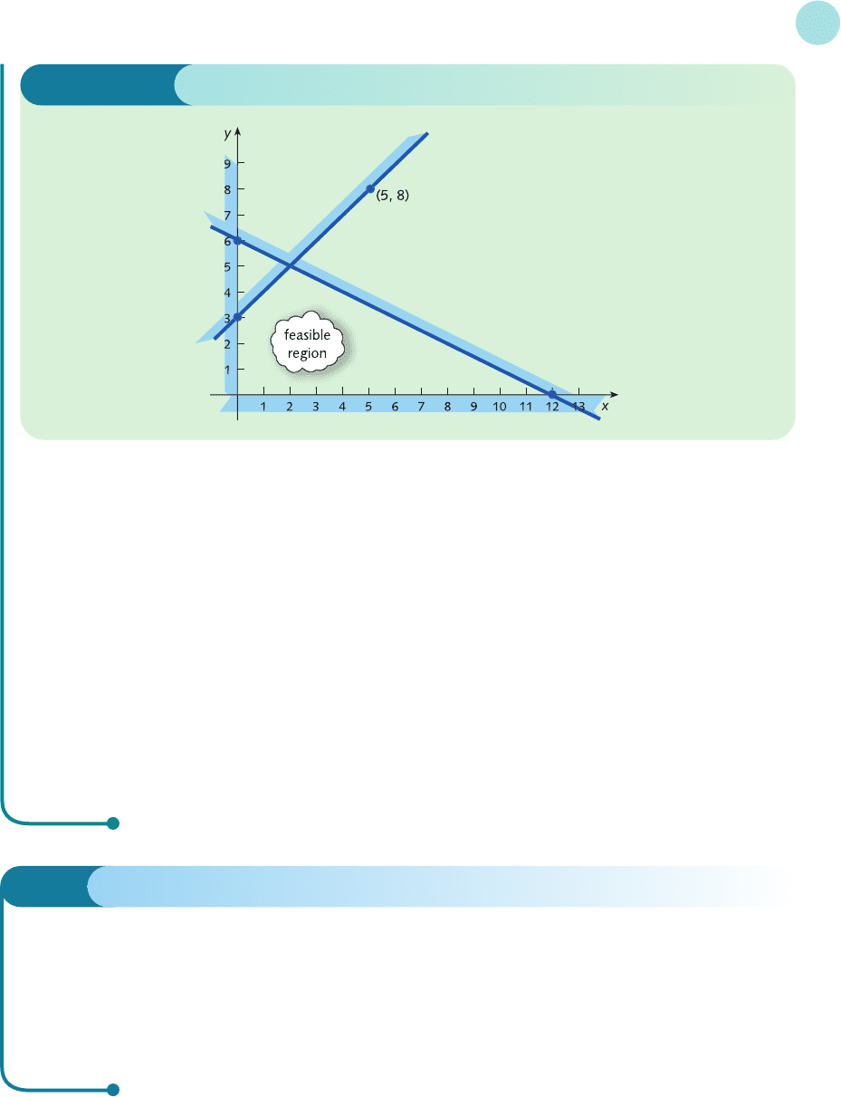
For the inequality
x + 2y ≤ 12
we need to sketch the line
x + 2y = 12
When x = 0 we get
2y = 12
and so y = 12/2 = 6.
When y = 0 we get
x = 12
The line passes through (0, 6) and (12, 0).
For a test point let us take (0, 0), since such a choice minimizes the amount of arithmetic that we have to
do. Substituting x = 0 and y = 0 into the inequality gives
0 + 2(0) ≤ 12
which is obviously true. Now the region containing the origin lies below the line, so we shade the region that
lies above it. This is indicated in Figure 8.6.
For the inequality
−x + y ≤ 3
we need to sketch the line
−x + y = 3
When x = 0 we get
y = 3
When y = 0 we get
−x = 3
and so x = 3/(−1) =−3.
Linear Programming
522
Figure 8.6
MFE_C08a.qxd 16/12/2005 10:47 Page 522
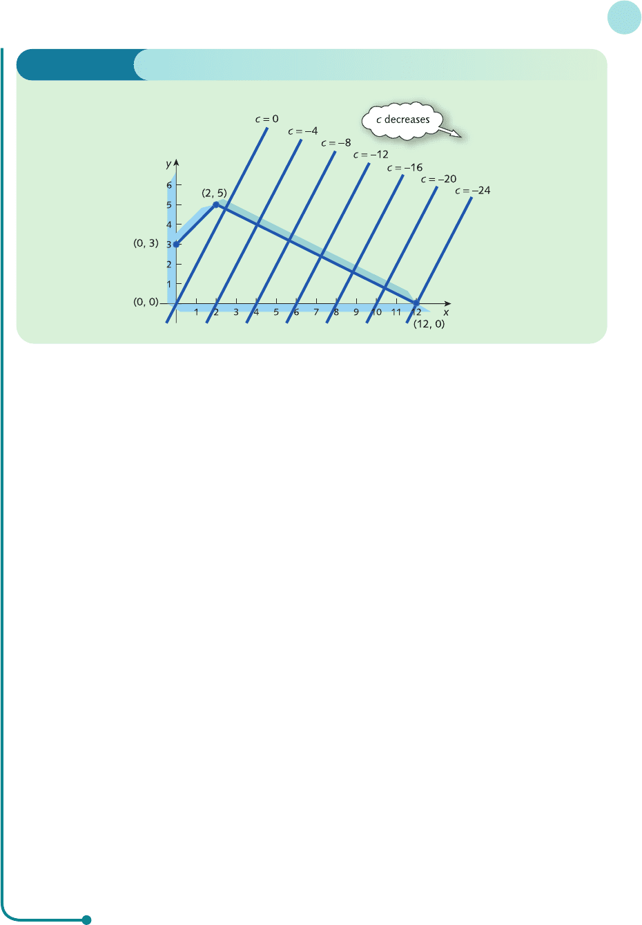
The line passes through (0, 3) and (−3, 0). Unfortunately, the second point does not lie on the diagram
as we have drawn it. At this stage we can either redraw the x axis to include −3 or we can try finding another
point on the line which does fit on the graph. For example, putting x = 5 gives
−5 + y = 3
so y = 3 + 5 = 8. Hence the line passes through (5, 8), which can now be plotted along with (0, 3) to sketch
the line. At the test point (0, 0) the inequality reads
−0 + 0 ≤ 3
which is obviously true. We are therefore interested in the region below the line, since this contains the ori-
gin. As usual we indicate this by shading the region on the other side. The complete picture is shown in
Figure 8.7.
Points (x, y) which satisfy all four inequalities must lie in the unshaded ‘hole’ in the middle. Incidentally,
this explains why we did not adopt the convention of shading the region of interest. Had we done so, our
task would have been to identify the most heavily shaded part of the diagram, which is not so easy.
8.1 • Graphical solution of linear programming problems
523
Practice Problem
2 Sketch the feasible region
x + 2y ≤ 10
−3x + y ≤ 10
x ≥ 0
y ≥ 0
Figure 8.7
We are now in a position to explain exactly what we mean by a linear programming prob-
lem and how such a problem can be solved graphically. We actually intend to describe two
slightly different methods of solution. One of these is fairly sophisticated and difficult to use,
while the other is more straightforward. The justification for bothering with the ‘harder’
MFE_C08a.qxd 16/12/2005 10:47 Page 523

method is that it provides the motivation for the ‘easier’ method. It also helps us to handle one
or two trickier problems that sometimes arise. We shall introduce both methods by concen-
trating on a specific example.
Linear Programming
524
Example
Solve the linear programming problem:
Minimize −2x + y
subject to the constraints
x + 2y ≤ 12
−x + y ≤ 3
x ≥ 0
y ≥ 0
Solution
In general, there are three ingredients making up a linear programming problem. Firstly, there are several
unknowns to be determined. In this example there are just two unknowns, x and y. Secondly, there is a
mathematical expression of the form
ax + by
which we want to either maximize or minimize. Such an expression is called an objective function. In this
example, a =−2, b = 1 and the problem is one of minimization. Finally, the unknowns x and y are subject
to a collection of linear inequalities. Quite often (but not always) two of the inequalities are x ≥ 0 and y ≥ 0.
These are referred to as non-negativity constraints. In this example there are a total of four constraints
including the non-negativity constraints.
Geometrically, points (x, y) which satisfy simultaneous linear inequalities define a feasible region in the co-
ordinate plane. In fact, for this particular problem, the feasible region has already been sketched in Figure 8.7.
The problem now is to try to identify that point inside the feasible region which minimizes the value
of the objective function. One naïve way of doing this might be to use trial and error: that is, we could
evaluate the objective function at every point within the region and choose the point which produces the
smallest value. For instance, (1, 1) lies in the region and when the values x = 1 and y = 1 are substituted into
−2x + y
we get
−2(1) + 1 =−1
Similarly we might try (3.4, 2.1), which produces
−2(3.4) + 2.1 =−4.7
which is an improvement, since −4.7 <−1.
The drawback of this approach is that there are infinitely many points inside the region, so it is going to
take a very long time before we can be certain of the solution! A more systematic approach is to superim-
pose, on top of the feasible region, the family of straight lines,
−2x + y = c
MFE_C08a.qxd 16/12/2005 10:47 Page 524
for various values of the constant c. Looking back at the objective function, you will notice that the number
c is precisely the thing that we want to minimize. That such an equation represents a straight line should
come as no surprise to you by now. Indeed, we know from the rearrangement
y = 2x + c
that the line has a slope of 2 with a y intercept of c. Consequently, all of these lines are parallel to each other,
their precise location being determined from the number c.
Now when y = 0 the equation reads
0 = 2x + c
and so has solution x =−c/2. Hence the line passes through the point (−c/2, 0). A selection of lines is
sketched in Figure 8.8 for values of c in the range 0 to −24. These have been sketched using the information
that they pass through (−c/2, 0) and have a slope of 2. Note that as c decreases from 0 to −24, the lines sweep
across the feasible region from left to right. Also, once c goes below −24 the lines no longer intersect this
region. The minimum value of c (which, you may remember, is just the value of the objective function) is
therefore −24. Moreover, when c =−24, the line
−2x + y = c
intersects the feasible region in exactly one point, namely (12, 0). This then must be the solution of our
problem. The point (12, 0) lies in the feasible region as required and because it also lies on the line
−2x + y =−24
we know that the corresponding value of the objective function is −24, which is the minimum value. Other
points in the feasible region also lie on lines
−2x + y = c
but with larger values of c.
8.1 • Graphical solution of linear programming problems
525
Figure 8.8
MFE_C08a.qxd 16/12/2005 10:47 Page 525

In the previous example, and in Practice Problem 3, the optimal value of the objective func-
tion is attained at one of the corners of the feasible region. This is not simply a coincidence. It
can be shown that the solution of any linear programming problem always occurs at one of the
corners. Consequently, the trial-and-error approach suggested earlier is not so naïve after all.
The only possible candidates for the answer are the corners and so only a finite number of
points need ever be examined. This method may be summarized:
Step 1
Sketch the feasible region.
Step 2
Identify the corners of the feasible region and find their coordinates.
Step 3
Evaluate the objective function at the corners and choose the one which has the maximum or
minimum value.
Returning to the previous example, we work as follows:
Step 1
The feasible region has already been sketched in Figure 8.7.
Step 2
There are four corners with coordinates (0, 0), (0, 3), (2, 5) and (12, 0).
Linear Programming
526
Practice Problem
3 Consider the linear programming problem
Maximize −x + y
subject to the constraints
3x + 4y ≤ 12
x ≥ 0
y ≥ 0
(a) Sketch the feasible region.
(b) Sketch, on the same diagram, the five lines
y = x + c
for c =−4, −2, 0, 1 and 3.
[Hint: lines of the form y = x + c have a slope of 1 and pass through the points (0, c) and (−c, 0).]
(c) Use your answers to part (b) to solve the given linear programming problem.
MFE_C08a.qxd 16/12/2005 10:47 Page 526

From this we see that the minimum occurs at (12, 0), at which the objective function is −24.
Incidentally, if we also require the maximum then this can be deduced without further effort.
From the table the maximum is 3, which occurs at (0, 3).
8.1 • Graphical solution of linear programming problems
527
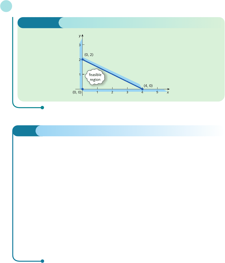
Corner Objective function
(0, 0) 5(0) + 3(0) = 0
(0, 2) 5(0) + 3(2) = 6
(4, 0) 5(4) + 3(0) = 20
Step 3
Corner Objective function
(0, 0) −2(0) + 0 = 0
(0, 3) −2(0) + 3 = 3
(2, 5) −2(2) + 5 = 1
(12, 0) −2(12) + 0 =−24
The maximum value of the objective function is 20, which occurs when x = 4 and y = 0.
Example
Solve the linear programming problem
Maximize 5x + 3y
subject to
2x + 4y ≤ 8
x ≥ 0
y ≥ 0
Solution
Step 1
The non-negativity constraints x ≥ 0 and y ≥ 0 indicate that the region is bounded by the coordinate axes in
the positive quadrant.
The line 2x + 4y = 8 passes through (0, 2) and (4, 0). Also, at the test point (0, 0) the inequality
2x + 4y ≤ 8
reads
0 ≤ 8
which is true. We are therefore interested in the region below the line, since this region contains the test
point, (0, 0). The feasible region is sketched in Figure 8.9 (overleaf).
Step 2
The feasible region is a triangle with three corners, (0, 0), (0, 2) and (4, 0).
Step 3
MFE_C08a.qxd 16/12/2005 10:47 Page 527
In Section 1.2 we showed you how to solve a system of simultaneous linear equations.
We discovered that such a system does not always have a unique solution. It is possible for a
problem to have either no solution or infinitely many solutions. An analogous situation arises
in linear programming. We conclude this section by considering two examples that illustrate
these special cases.
Linear Programming
528
Figure 8.9
Practice Problems
4 Solve the linear programming problem
Minimize x − y
subject to
2x + y ≤ 2
x ≥ 0
y ≥ 0
5 Solve the linear programming problem
Maximize 3x + 5y
subject to
x + 2y ≤ 10
3x + y ≤ 10
x ≥ 0
y ≥ 0
[Hint: you might find your answer to Practice Problem 2 useful.]
MFE_C08a.qxd 16/12/2005 10:47 Page 528

This time, however, the maximum value is 4, which actually occurs at two corners, (0, 2) and (4, 0). This
shows that the problem does not have a unique solution. To explain what is going on here we return to the
method introduced at the beginning of this section. We superimpose the family of lines obtained by setting
the objective function equal to some constant, c. The parallel lines
x + 2y = c
pass through the points (0, c/2) and (c, 0).
A selection of lines is sketched in Figure 8.10 (overleaf ) for values of c between 0 and 4. These particular
values are chosen since they produce lines that cross the feasible region. As c increases, the lines sweep across
the region from left to right. Moreover, when c goes above 4 the lines no longer intersect the region. The
maximum value that c (that is, the objective function) can take is therefore 4. However, instead of the line
x + 2y = 4
intersecting the region at only one point, it intersects along a whole line segment of points. Any point on
the line joining the two corners (0, 2) and (4, 0) will be a solution. This follows because any point on this
line segment lies in the feasible region and the corresponding value of the objective function on this line
is 4, which is the maximum value.
8.1 • Graphical solution of linear programming problems
529
Corner Objective function
(0, 0) 0 + 2(0) = 0
(0, 2) 0 + 2(2) = 4
(4, 0) 4 + 2(0) = 4
Example
Solve the linear programming problem
Maximize x + 2y
subject to
2x + 4y ≤ 8
x ≥ 0
y ≥ 0
Solution
Step 1
The feasible region is identical to the one sketched in Figure 8.9 for the previous worked example.
Step 2
As before, the feasible region has three corners, (0, 0), (0, 2) and (4, 0).
Step 3
MFE_C08a.qxd 16/12/2005 10:47 Page 529